![]()

Tutorial 5: Model Selection: Bias-variance trade-off#
Week 1, Day 2: Model Fitting
By Neuromatch Academy
Content creators: Pierre-Étienne Fiquet, Anqi Wu, Alex Hyafil with help from Ella Batty
Content reviewers: Lina Teichmann, Patrick Mineault, Michael Waskom
Production editors: Spiros Chavlis
Tutorial Objectives#
Estimated timing of tutorial: 25 minutes
This is Tutorial 5 of a series on fitting models to data. We start with simple linear regression, using least squares optimization (Tutorial 1) and Maximum Likelihood Estimation (Tutorial 2). We will use bootstrapping to build confidence intervals around the inferred linear model parameters (Tutorial 3). We’ll finish our exploration of regression models by generalizing to multiple linear regression and polynomial regression (Tutorial 4). We end by learning how to choose between these various models. We discuss the bias-variance trade-off (Tutorial 5) and Cross Validation for model selection (Tutorial 6).
In this tutorial, we will learn about the bias-variance tradeoff and see it in action using polynomial regression models.
Tutorial objectives:
Understand difference between test and train data
Compare train and test error for models of varying complexity
Understand how bias-variance tradeoff relates to what model we choose
Setup#
Install and import feedback gadget#
Show code cell source
# @title Install and import feedback gadget

!pip3 install vibecheck datatops --quiet

from vibecheck import DatatopsContentReviewContainer
def content_review(notebook_section: str):
    return DatatopsContentReviewContainer(
        "",  # No text prompt
        notebook_section,
        {
            "url": "https://pmyvdlilci.execute-api.us-east-1.amazonaws.com/klab",
            "name": "neuromatch_cn",
            "user_key": "y1x3mpx5",
        },
    ).render()


feedback_prefix = "W1D2_T5"
# Imports
import numpy as np
import matplotlib.pyplot as plt
Figure Settings#
Show code cell source
# @title Figure Settings
import logging
logging.getLogger('matplotlib.font_manager').disabled = True

%config InlineBackend.figure_format = 'retina'
plt.style.use("https://raw.githubusercontent.com/NeuromatchAcademy/course-content/main/nma.mplstyle")
Plotting Functions#
Show code cell source
# @title Plotting Functions

def plot_MSE_poly_fits(mse_train, mse_test, max_order):
  """
    Plot the MSE values for various orders of polynomial fits on the same bar
    graph

    Args:
      mse_train (ndarray): an array of MSE values for each order of polynomial fit
      over the training data
      mse_test (ndarray): an array of MSE values for each order of polynomial fit
      over the test data
      max_order (scalar): max order of polynomial fit
  """
  fig, ax = plt.subplots()
  width = .35

  ax.bar(np.arange(max_order + 1) - width / 2,
         mse_train, width, label="train MSE")
  ax.bar(np.arange(max_order + 1) + width / 2,
         mse_test , width, label="test MSE")

  ax.legend()
  ax.set(xlabel='Polynomial order', ylabel='MSE',
         title='Comparing polynomial fits')
  plt.show()
Helper functions#
Show code cell source
# @title Helper functions

def ordinary_least_squares(x, y):
  """Ordinary least squares estimator for linear regression.

  Args:
    x (ndarray): design matrix of shape (n_samples, n_regressors)
    y (ndarray): vector of measurements of shape (n_samples)

  Returns:
    ndarray: estimated parameter values of shape (n_regressors)
  """

  return np.linalg.inv(x.T @ x) @ x.T @ y


def make_design_matrix(x, order):
  """Create the design matrix of inputs for use in polynomial regression

  Args:
    x (ndarray): input vector of shape (n_samples)
    order (scalar): polynomial regression order

  Returns:
    ndarray: design matrix for polynomial regression of shape (samples, order+1)
  """

  # Broadcast to shape (n x 1) so dimensions work
  if x.ndim == 1:
    x = x[:, None]

  #if x has more than one feature, we don't want multiple columns of ones so we assign
  # x^0 here
  design_matrix = np.ones((x.shape[0],1))

  # Loop through rest of degrees and stack columns
  for degree in range(1, order+1):
      design_matrix = np.hstack((design_matrix, x**degree))

  return design_matrix


def solve_poly_reg(x, y, max_order):
  """Fit a polynomial regression model for each order 0 through max_order.

  Args:
    x (ndarray): input vector of shape (n_samples)
    y (ndarray): vector of measurements of shape (n_samples)
    max_order (scalar): max order for polynomial fits

  Returns:
    dict: fitted weights for each polynomial model (dict key is order)
  """

  # Create a dictionary with polynomial order as keys, and np array of theta
  # (weights) as the values
  theta_hats = {}

  # Loop over polynomial orders from 0 through max_order
  for order in range(max_order+1):

    X = make_design_matrix(x, order)
    this_theta = ordinary_least_squares(X, y)

    theta_hats[order] = this_theta

  return theta_hats
Section 1: Train vs test data#
Estimated timing to here from start of tutorial: 8 min
The data used for the fitting procedure for a given model is the training data. In tutorial 4, we computed MSE on the training data of our polynomial regression models and compared training MSE across models. An additional important type of data is test data. This is held-out data that is not used (in any way) during the fitting procedure. When fitting models, we often want to consider both the train error (the quality of prediction on the training data) and the test error (the quality of prediction on the test data) as we will see in the next section.
Video 1: Bias Variance Tradeoff#
Submit your feedback#
Show code cell source
# @title Submit your feedback
content_review(f"{feedback_prefix}_Bias_Variance_Tradeoff_Video")
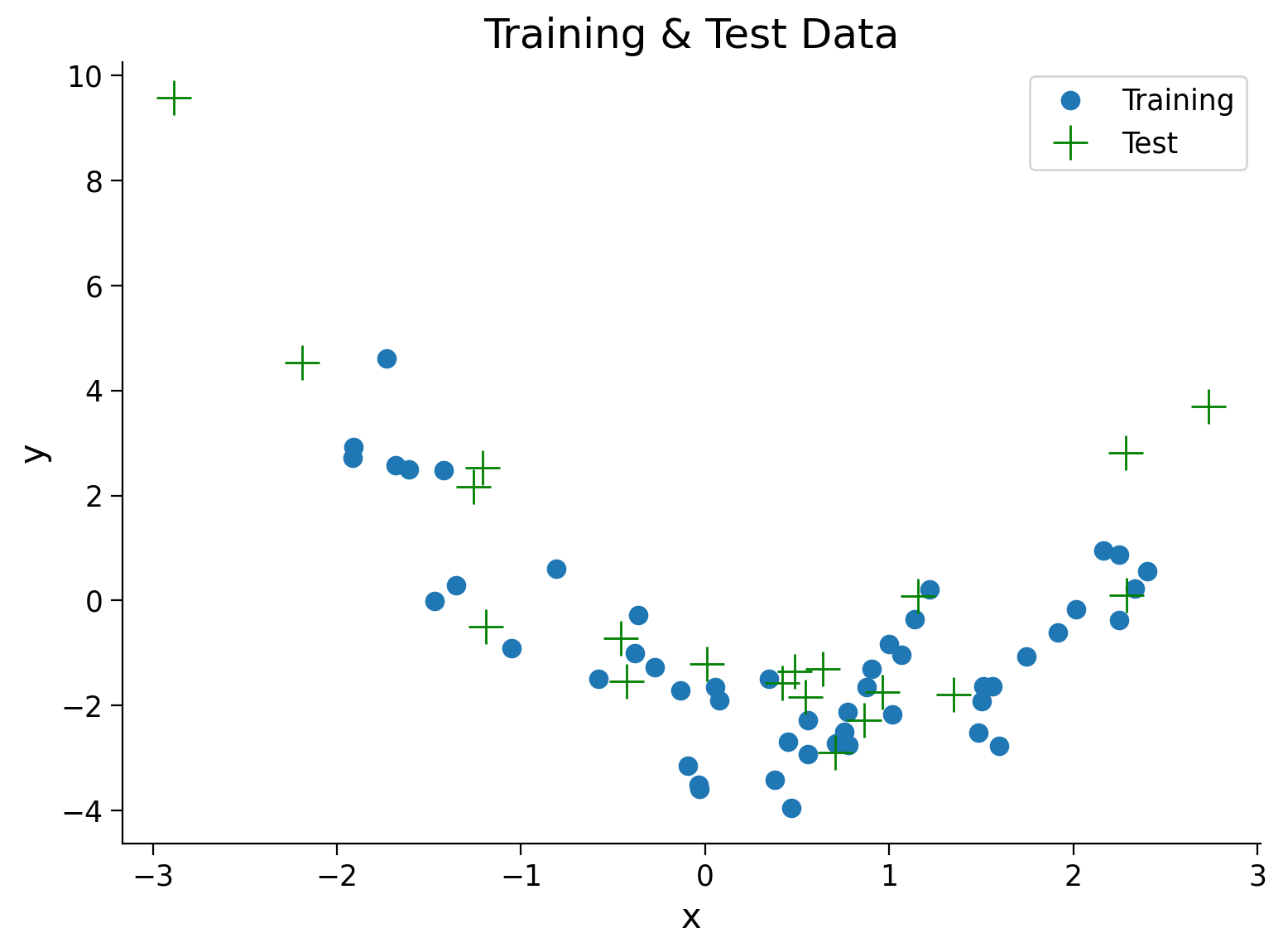
We will generate some noisy data for use in this tutorial using a similar process as in Tutorial 4. However, now we will also generate test data. We want to see how our model generalizes beyond the range of values seen in the training phase. To accomplish this, we will generate x from a wider range of values ([-3, 3]). We then plot the train and test data together.
Execute this cell to simulate both training and test data
Show code cell source
# @markdown Execute this cell to simulate both training and test data

### Generate training data
np.random.seed(0)
n_train_samples = 50
x_train = np.random.uniform(-2, 2.5, n_train_samples) # sample from a uniform distribution over [-2, 2.5)
noise = np.random.randn(n_train_samples) # sample from a standard normal distribution
y_train =  x_train**2 - x_train - 2 + noise

### Generate testing data
n_test_samples = 20
x_test = np.random.uniform(-3, 3, n_test_samples) # sample from a uniform distribution over [-2, 2.5)
noise = np.random.randn(n_test_samples) # sample from a standard normal distribution
y_test =  x_test**2 - x_test - 2 + noise

## Plot both train and test data
fig, ax = plt.subplots()
plt.title('Training & Test Data')
plt.plot(x_train, y_train, '.', markersize=15, label='Training')
plt.plot(x_test, y_test, 'g+', markersize=15, label='Test')
plt.legend()
plt.xlabel('x')
plt.ylabel('y');
Section 2: Bias-variance tradeoff#
Estimated timing to here from start of tutorial: 10 min
Click here for text recap of video
Finding a good model can be difficult. One of the most important concepts to keep in mind when modeling is the bias-variance tradeoff.
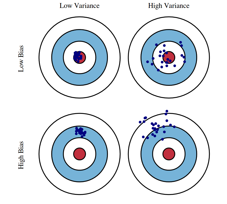
Bias is the difference between the prediction of the model and the corresponding true output variables you are trying to predict. Models with high bias will not fit the training data well since the predictions are quite different from the true data. These high bias models are overly simplified - they do not have enough parameters and complexity to accurately capture the patterns in the data and are thus underfitting.
Variance refers to the variability of model predictions for a given input. Essentially, do the model predictions change a lot with changes in the exact training data used? Models with high variance are highly dependent on the exact training data used - they will not generalize well to test data. These high variance models are overfitting to the data.
In essence:
High bias, low variance models have high train and test error.
Low bias, high variance models have low train error, high test error
Low bias, low variance models have low train and test error
As we can see from this list, we ideally want low bias and low variance models! These goals can be in conflict though - models with enough complexity to have low bias also tend to overfit and depend on the training data more. We need to decide on the correct tradeoff.
In this section, we will see the bias-variance tradeoff in action with polynomial regression models of different orders.
Graphical illustration of bias and variance. (Source: http://scott.fortmann-roe.com/docs/BiasVariance.html)
We will first fit polynomial regression models of orders 0-5 on our simulated training data just as we did in Tutorial 4.
Execute this cell to estimate theta_hats
Show code cell source
# @markdown Execute this cell to estimate theta_hats
max_order = 5
theta_hats = solve_poly_reg(x_train, y_train, max_order)
Coding Exercise 2: Compute and compare train vs test error#
We will use MSE as our error metric again. Compute MSE on training data (\(x_{train},y_{train}\)) and test data (\(x_{test}, y_{test}\)) for each polynomial regression model (orders 0-5). Since you already developed code in T4 Exercise 4 for making design matrices and evaluating fit polynomials, we have ported that here into the functions make_design_matrix and evaluate_poly_reg for your use.
Please think about it after completing the exercise before reading the following text! Do you think the order 0 model has high or low bias? High or low variance? How about the order 5 model?
Execute this cell for function evalute_poly_reg
Show code cell source
# @markdown Execute this cell for function `evalute_poly_reg`

def evaluate_poly_reg(x, y, theta_hats, max_order):
  """ Evaluates MSE of polynomial regression models on data

  Args:
    x (ndarray): input vector of shape (n_samples)
    y (ndarray): vector of measurements of shape (n_samples)
    theta_hats (dict):  fitted weights for each polynomial model (dict key is order)
    max_order (scalar): max order of polynomial fit

  Returns
    (ndarray): mean squared error for each order, shape (max_order)
  """

  mse = np.zeros((max_order + 1))
  for order in range(0, max_order + 1):
    X_design = make_design_matrix(x, order)
    y_hat = np.dot(X_design, theta_hats[order])
    residuals = y - y_hat
    mse[order] = np.mean(residuals ** 2)

  return mse
def compute_mse(x_train, x_test, y_train, y_test, theta_hats, max_order):
"""Compute MSE on training data and test data.
Args:
x_train(ndarray): training data input vector of shape (n_samples)
x_test(ndarray): test data input vector of shape (n_samples)
y_train(ndarray): training vector of measurements of shape (n_samples)
y_test(ndarray): test vector of measurements of shape (n_samples)
theta_hats(dict): fitted weights for each polynomial model (dict key is order)
max_order (scalar): max order of polynomial fit
Returns:
ndarray, ndarray: MSE error on training data and test data for each order
"""
#######################################################
## TODO for students: calculate mse error for both sets
## Hint: look back at tutorial 5 where we calculated MSE
# Fill out function and remove
raise NotImplementedError("Student exercise: calculate mse for train and test set")
#######################################################
mse_train = ...
mse_test = ...
return mse_train, mse_test
# Compute train and test MSE
mse_train, mse_test = compute_mse(x_train, x_test, y_train, y_test, theta_hats, max_order)
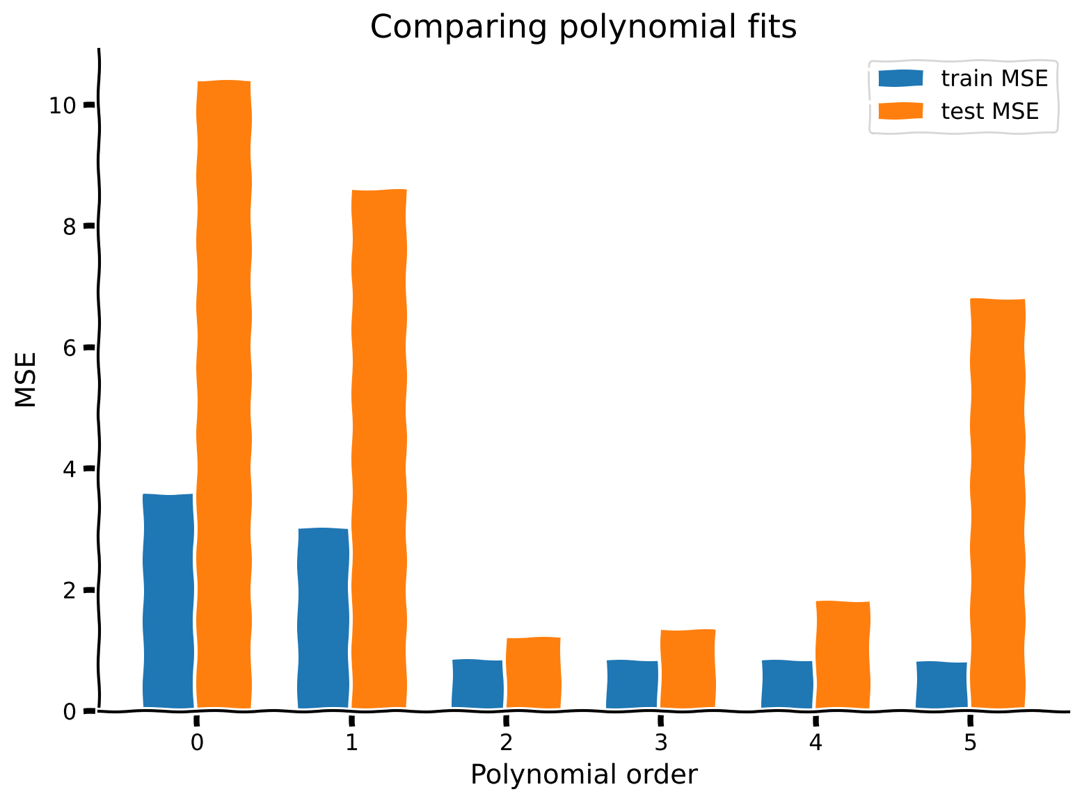
# Visualize
plot_MSE_poly_fits(mse_train, mse_test, max_order)
Example output:
Submit your feedback#
Show code cell source
# @title Submit your feedback
content_review(f"{feedback_prefix}_Compute_train_vs_test_error_Exercise")
As we can see from the plot above, more complex models (higher order polynomials) have lower MSE for training data. The overly simplified models (orders 0 and 1) have high MSE on the training data. As we add complexity to the model, we go from high bias to low bias.
The MSE on test data follows a different pattern. The best test MSE is for an order 2 model - this makes sense as the data was generated with an order 2 model. Both simpler models and more complex models have higher test MSE.
So to recap:
Order 0 model: High bias, low variance
Order 5 model: Low bias, high variance
Order 2 model: Just right, low bias, low variance
Summary#
Estimated timing of tutorial: 25 minutes
Training data is the data used for fitting, test data is held-out data.
We need to strike the right balance between bias and variance. Ideally we want to find a model with optimal model complexity that has both low bias and low variance
Too complex models have low bias and high variance.
Too simple models have high bias and low variance.
Note
Bias and variance are very important concepts in modern machine learning, but it has recently been observed that they do not necessarily trade off (see for example the phenomenon and theory of “double descent”)
Further readings:
The elements of statistical learning by Hastie, Tibshirani and Friedman
Bonus#
Bonus Exercise: Proof of bias-variance decomposition#
Prove the bias-variance decomposition for MSE
where
and
Click here for a hint
Use the equation:
Submit your feedback#
Show code cell source
# @title Submit your feedback
content_review(f"{feedback_prefix}_Proof_bias_variance_for_MSE_Bonus_Exercise")