Tutorial 2: Learning to Act: Multi-Armed Bandits

Tutorial 2: Learning to Act: Multi-Armed Bandits#

Week 3, Day 4: Reinforcement Learning

By Neuromatch Academy

Content creators: Marcelo G Mattar, Eric DeWitt, Matt Krause, Matthew Sargent, Anoop Kulkarni, Sowmya Parthiban, Feryal Behbahani, Jane Wang

Content reviewers: Ella Batty, Byron Galbraith, Michael Waskom, Ezekiel Williams, Mehul Rastogi, Lily Cheng, Roberto Guidotti, Arush Tagade, Kelson Shilling-Scrivo

Production editors: Gagana B, Spiros Chavlis

Tutorial Objectives#

Estimated timing of tutorial: 45 min

In this tutorial we will model the simplest types of acting agents. An acting agent can affect how much reward it receives, so it must learn how to identify the actions that lead to the most reward. You will use ‘bandits’ to understand the fundamentals of how a policy interacts with the learning algorithm in reinforcement learning.

You will understand the fundamental tradeoff between exploration and exploitation in a policy.
You will understand how the learning rate interacts with exploration to find the best available action.

Setup#

Install and import feedback gadget#

# Imports
import numpy as np
import matplotlib.pyplot as plt

Figure Settings#

Plotting Functions#

Section 1: Multi-Armed Bandits#

Video 1: Multi-Armed Bandits#

Submit your feedback#

Consider the following learning problem. You are faced repeatedly with a choice among \(k\) different options, or actions. After each choice you receive a reward signal in the form of a numerical value, where the larger value is the better. Your objective is to maximize the expected total reward over some time period, for example, over 1000 action selections, or time steps.

This is the original form of the k-armed bandit problem. This name derives from the colloquial name for a slot machine, the “one-armed bandit”, because it has the one lever to pull, and it is often rigged to take more money than it pays out over time. The multi-armed bandit extension is to imagine, for instance, that you are faced with multiple slot machines that you can play, but only one at a time. Which machine should you play, i.e., which arm should you pull, which action should you take, at any given time to maximize your total payout.

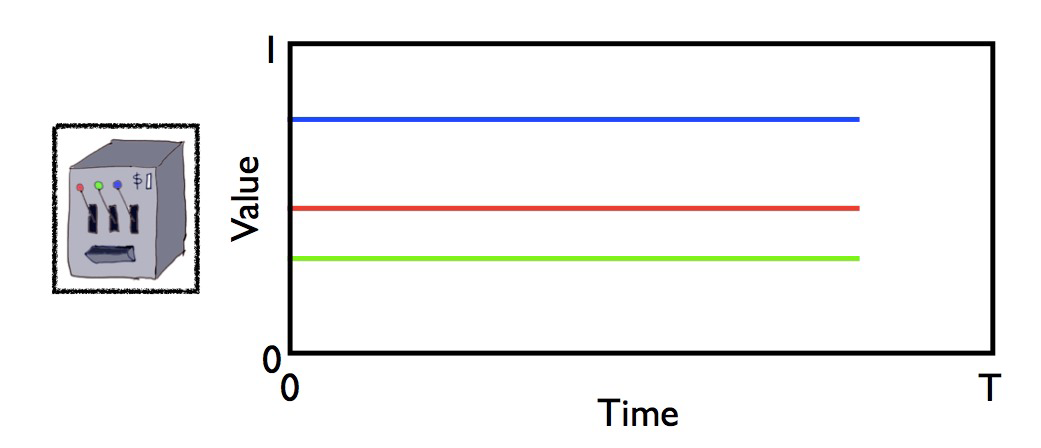
While there are many different levels of sophistication and assumptions in how the rewards are determined, we will consider here the simple scenario where each action results in a reward drawn from a different Gaussian distribution with unknown mean and unit variance. Since each action is associated with a different mean reward, the goal of the agent is to find the action with highest mean. But since the rewards are noisy (the corresponding Gaussians have unit variance), those means cannot be determined from a single observed reward.

This problem setting is referred to as the environment. We will solve this optimization problem with an agent, in this case an algorithm that takes in rewards and returns actions.

Section 2: Choosing an Action#

Estimated timing to here from start of tutorial: 10 min

The first thing our agent needs to be able to do is choose which arm to pull. The strategy for choosing actions based on our expectations is called a policy (often denoted \(\pi\)). We could have a random policy – just pick an arm at random each time – though this doesn’t seem likely to be capable of optimizing our reward. We want some intentionality, and to do that we need a way of describing our beliefs about the arms’ reward potential. We do this with an action-value function

(442)#\[\begin{equation} q(a) = \mathbb{E} [r_{t} | a_{t} = a] \end{equation}\]

where the value \(q\) for taking action \(a \in A\) at time \(t\) is equal to the expected value of the reward \(r_t\) given that we took action \(a\) at that time. In practice, this is often represented as an array of values, where each action’s value is a different element in the array.

Great, now that we have a way to describe our beliefs about the values each action should return, let’s come up with a policy.

An obvious choice would be to take the action with the highest expected value. This is referred to as the greedy policy

(443)#\[\begin{equation} a_{t} = \underset{a}{\operatorname{argmax}} \; q_{t} (a) \end{equation}\]

where our choice action is the one that maximizes the current value function.

So far so good, but it can’t be this easy. And, in fact, the greedy policy does have a fatal flaw: it easily gets trapped in local maxima. It never explores to see what it hasn’t seen before if one option is already better than the others. This leads us to a fundamental challenge in coming up with effective policies.

The Exploitation-Exploration Dilemma

If we never try anything new, if we always stick to the safe bet, we don’t know what we are missing. Sometimes we aren’t missing much of anything, and regret not sticking with our preferred choice, yet other times we stumble upon something new that was way better than we thought.

This is the exploitation-exploration dilemma: do you go with your best choice now, or risk the less certain option with the hope of finding something better. Too much exploration, however, means you may end up with a sub-optimal reward once it’s time to stop.

In order to avoid getting stuck in local minima while also maximizing reward, effective policies need some way to balance between these two aims.

A simple extension to our greedy policy is to add some randomness. For instance, a coin flip – heads we take the best choice now, tails we pick one at random. This is referred to as the \(\epsilon\)-greedy policy:

(444)#\[\begin{equation} P (a_{t} = a) = \begin{cases} 1 - \epsilon + \epsilon/N & \quad \text{if } a_{t} = \underset{a}{\operatorname{argmax}} \; q_{t} (a) \\ \epsilon/N & \quad \text{else} \end{cases} \end{equation}\]

which is to say that with probability 1 - \(\epsilon\) for \(\epsilon \in [0,1]\) we select the greedy choice, and otherwise we select an action at random (including the greedy option).

Despite its relative simplicity, the epsilon-greedy policy is quite effective, which leads to its general popularity.

Coding Exercise 2: Implement Epsilon-Greedy#

Referred to in video as Exercise 1

In this exercise you will implement the epsilon-greedy algorithm for deciding which action to take from a set of possible actions given their value function and a probability \(\epsilon\) of simply choosing one at random.

TIP: You may find np.random.random, np.random.choice, and np.argmax useful here.

def epsilon_greedy(q, epsilon):
  """Epsilon-greedy policy: selects the maximum value action with probability
  (1-epsilon) and selects randomly with epsilon probability.

  Args:
    q (ndarray): an array of action values
    epsilon (float): probability of selecting an action randomly

  Returns:
    int: the chosen action
  """
  #####################################################################
  ## TODO for students: implement the epsilon greedy decision algorithm
  # Fill out function and remove
  raise NotImplementedError("Student exercise: implement the epsilon greedy decision algorithm")
  #####################################################################
  # write a boolean expression that determines if we should take the best action
  be_greedy = ...

  if be_greedy:

    # write an expression for selecting the best action from the action values
    action = ...

  else:

    # write an expression for selecting a random action
    action = ...

  return action


# Set parameters
q = [-2, 5, 0, 1]
epsilon = 0.1

# Visualize
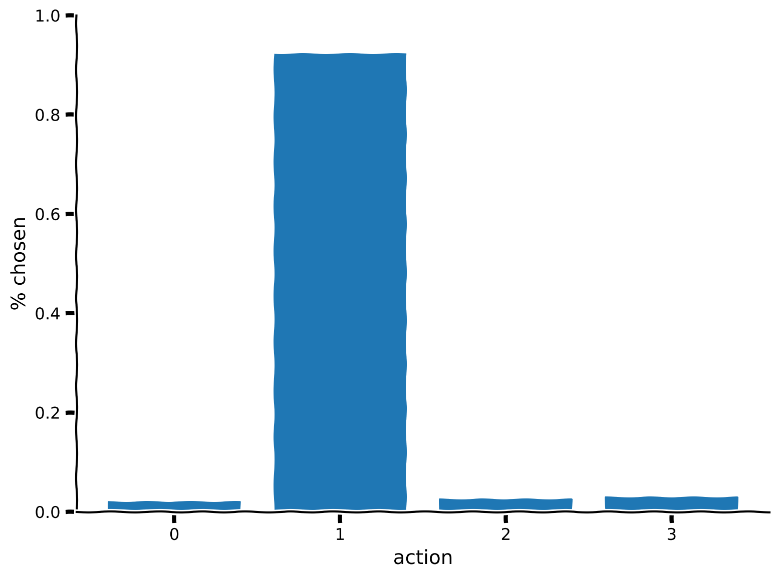
plot_choices(q, epsilon, epsilon_greedy)

Click for solution

Example output:

Submit your feedback#

This is what we should expect, that the action with the largest value (action 1) is selected about (1-\(\epsilon\)) of the time, or 90% for \(\epsilon = 0.1\), and the remaining 10% is split evenly amongst the other options. Use the demo below to explore how changing \(\epsilon\) affects the distribution of selected actions.

Interactive Demo 2: Changing Epsilon#

Epsilon is our one parameter for balancing exploitation and exploration. Given a set of values \(q = [-2, 5, 0, 1]\), use the widget below to see how changing \(\epsilon\) influences our selection of the max value 5 (action = 1) vs the others.

At the extremes of its range (0 and 1), the \(\epsilon\)-greedy policy reproduces two other policies. What are they?

Make sure you execute this cell to enable the widget!

Click for solution

Submit your feedback#

Section 3: Learning from Rewards#

Estimated timing to here from start of tutorial: 25 min

Now that we have a policy for deciding what to do, how do we learn from our actions?

One way to do this is just keep a record of every result we ever got and use the averages for each action. If we have a potentially very long running episode, the computational cost of keeping all these values and recomputing the mean over and over again isn’t ideal. Instead we can use a streaming mean calculation, which looks like this:

(445)#\[\begin{equation} q_{t+1}(a) \leftarrow q_{t}(a) + \frac{1}{n_t} (r_{t} - q_{t}(a)) \end{equation}\]

where our action-value function \(q_t(a)\) is the mean of the rewards seen so far, \(n_t\) is the number of actions taken by time \(t\), and \(r_t\) is the reward just received for taking action \(a\).

This still requires us to remember how many actions we’ve taken, so let’s generalize this a bit further and replace the action total with a general parameter \(\alpha\), which we will call the learning rate

(446)#\[\begin{equation} q_{t+1}(a) \leftarrow q_{t}(a) + \alpha (r_{t} - q_{t}(a)). \end{equation}\]

Coding Exercise 3: Updating Action Values#

Referred to in video as Exercise 2

In this exercise you will implement the action-value update rule above. The function will take in the action-value function represented as an array q, the action taken, the reward received, and the learning rate, alpha. The function will return the updated value for the selection action.

def update_action_value(q, action, reward, alpha):
  """ Compute the updated action value given the learning rate and observed
  reward.

  Args:
    q (ndarray): an array of action values
    action (int): the action taken
    reward (float): the reward received for taking the action
    alpha (float): the learning rate

  Returns:
    float: the updated value for the selected action
  """
  #####################################################
  ## TODO for students: compute the action value update
  # Fill out function and remove
  raise NotImplementedError("Student exercise: compute the action value update")
  #####################################################

  # Write an expression for the updated action value
  value = ...

  return value


# Set parameters
q = [-2, 5, 0, 1]
action = 2
print(f"Original q({action}) value = {q[action]}")

# Update action
q[action] = update_action_value(q, 2, 10, 0.01)
print(f"Updated q({action}) value = {q[action]}")

You should see

Original q(2) value = 0
Updated q(2) value = 0.1

Click for solution

Submit your feedback#

Section 4: Solving Multi-Armed Bandits#

Estimated timing to here from start of tutorial: 31 min

Now that we have both a policy and a learning rule, we can combine these to solve our original multi-armed bandit task. Recall that we have some number of arms that give rewards drawn from Gaussian distributions with unknown mean and unit variance, and our goal is to find the arm with the highest mean.

First, let’s see how we will simulate this environment by reading through the annotated code below.

def multi_armed_bandit(n_arms, epsilon, alpha, n_steps):
  """ A Gaussian multi-armed bandit using an epsilon-greedy policy. For each
  action, rewards are randomly sampled from normal distribution, with a mean
  associated with that arm and unit variance.

  Args:
    n_arms (int): number of arms or actions
    epsilon (float): probability of selecting an action randomly
    alpha (float): the learning rate
    n_steps (int): number of steps to evaluate

  Returns:
    dict: a dictionary containing the action values, actions, and rewards from
    the evaluation along with the true arm parameters mu and the optimality of
    the chosen actions.
  """
  # Gaussian bandit parameters
  mu = np.random.normal(size=n_arms)

  # Evaluation and reporting state
  q = np.zeros(n_arms)
  qs = np.zeros((n_steps, n_arms))
  rewards = np.zeros(n_steps)
  actions = np.zeros(n_steps)
  optimal = np.zeros(n_steps)

  # Run the bandit
  for t in range(n_steps):

    # Choose an action
    action = epsilon_greedy(q, epsilon)
    actions[t] = action

    # Compute rewards for all actions
    all_rewards = np.random.normal(mu)

    # Observe the reward for the chosen action
    reward = all_rewards[action]
    rewards[t] = reward

    # Was it the best possible choice?
    optimal_action = np.argmax(all_rewards)
    optimal[t] = action == optimal_action

    # Update the action value
    q[action] = update_action_value(q, action, reward, alpha)
    qs[t] = q

  results = {
      'qs': qs,
      'actions': actions,
      'rewards': rewards,
      'mu': mu,
      'optimal': optimal
  }

  return results

We can use our multi-armed bandit method to evaluate how our epsilon-greedy policy and learning rule perform at solving the task. First we will set our environment to have 10 arms and our agent parameters to \(\epsilon=0.1\) and \(\alpha=0.01\). In order to get a good sense of the agent’s performance, we will run the episode for 1000 steps.

Execute to see visualization

Alright, we got some rewards that are kind of all over the place, but the agent seemed to settle in on the first arm as the preferred choice of action relatively quickly. Let’s see how well we did at recovering the true means of the Gaussian random variables behind the arms.

Execute to see visualization

Well, we seem to have found a very good estimate for action 0, but most of the others are not great. In fact, we can see the effect of the local maxima trap at work – the greedy part of our algorithm locked onto action 0, which is actually the 2nd best choice to action 6. Since these are the means of Gaussian random variables, we can see that the overlap between the two would be quite high, so even if we did explore action 6, we may draw a sample that is still lower than our estimate for action 0.

However, this was just one choice of parameters. Perhaps there is a better combination?

Interactive Demo 4: Changing Epsilon and Alpha#

Referred to in video as Exercise 3

Use the widget below to explore how varying the values of \(\epsilon\) (exploitation-exploration tradeoff), \(\alpha\) (learning rate), and even the number of actions \(k\), changes the behavior of our agent.

Make sure you execute this cell to enable the widget!

While we can see how changing the epsilon and alpha values impact the agent’s behavior, this doesn’t give us a great sense of which combination is optimal. Due to the stochastic nature of both our rewards and our policy, a single trial run isn’t sufficient to give us this information. Let’s run multiple trials and compare the average performance.

First we will look at different values for \(\epsilon \in [0.0, 0.1, 0.2]\) to a fixed \(\alpha=0.1\). We will run 200 trials as a nice balance between speed and accuracy.

Execute this cell to see visualization

On the left we have plotted the average reward over time, and we see that while \(\epsilon=0\) (the greedy policy) does well initially, \(\epsilon=0.1\) starts to do slightly better in the long run, while \(\epsilon=0.2\) does the worst. Looking on the right, we see the percentage of times the optimal action (the best possible choice at time \(t\)) was taken, and here again we see a similar pattern of \(\epsilon=0.1\) starting out a bit slower but eventually having a slight edge in the longer run.

We can also do the same for the learning rates. We will evaluate \(\alpha \in [0.01, 0.1, 1.0]\) to a fixed \(\epsilon=0.1\).

Execute this cell to see visualization

Again we see a balance between an effective learning rate. \(\alpha=0.01\) is too weak to quickly incorporate good values, while \(\alpha=1\) is too strong likely resulting in high variance in values due to the Gaussian nature of the rewards.

Submit your feedback#

Summary#

Estimated timing of tutorial: 45 min

In this tutorial you implemented both the epsilon-greedy decision algorithm and a learning rule for solving a multi-armed bandit scenario. You saw how balancing exploitation and exploration in action selection is critical in finding optimal solutions. You also saw how choosing an appropriate learning rate determines how well an agent can generalize the information they receive from rewards.

Tutorial 2: Learning to Act: Multi-Armed Bandits

Contents

Tutorial 2: Learning to Act: Multi-Armed Bandits#

Tutorial Objectives#

Setup#

Install and import feedback gadget#

Figure Settings#

Plotting Functions#

Section 1: Multi-Armed Bandits#

Video 1: Multi-Armed Bandits#

Submit your feedback#

Section 2: Choosing an Action#

Coding Exercise 2: Implement Epsilon-Greedy#

Submit your feedback#

Interactive Demo 2: Changing Epsilon#

Submit your feedback#

Section 3: Learning from Rewards#

Coding Exercise 3: Updating Action Values#

Submit your feedback#

Section 4: Solving Multi-Armed Bandits#

Interactive Demo 4: Changing Epsilon and Alpha#

Submit your feedback#

Summary#