Tutorial 1: Decoding Neural Responses

Tutorial 1: Decoding Neural Responses#

Week 1, Day 5: Deep Learning

By Neuromatch Academy

Content creators: Jorge A. Menendez, Carsen Stringer

Content reviewers: Roozbeh Farhoodi, Madineh Sarvestani, Kshitij Dwivedi, Spiros Chavlis, Ella Batty, Michael Waskom

Production editors: Spiros Chavlis

Tutorial Objectives#

Estimated timing of tutorial: 1 hr, 20 minutes

In this tutorial, we’ll use deep learning to decode stimulus information from the responses of sensory neurons. Specifically, we’ll look at the activity of ~20,000 neurons in the mouse primary visual cortex responding to oriented gratings recorded in this study. Our task will be to decode the orientation of the presented stimulus from the responses of the whole population of neurons. We could do this in a number of ways, but here we’ll use deep learning. Deep learning is particularly well-suited to this problem for a number of reasons:

The data are very high-dimensional: the neural response to a stimulus is a ~20,000 dimensional vector. Many machine learning techniques fail in such high dimensions, but deep learning actually thrives in this regime, as long as you have enough data (which we do here!).
As you’ll be able to see below, different neurons can respond quite differently to stimuli. This complex pattern of responses will, therefore, require non-linear methods to be decoded, which we can easily do with non-linear activation functions in deep networks.
Deep learning architectures are highly flexible, meaning we can easily adapt the architecture of our decoding model to optimize decoding. Here, we’ll focus on a single architecture, but you’ll see that it can easily be modified with few changes to the code.

More concretely, our goal will be learn how to:

Build a deep feed-forward network using PyTorch
Evaluate the network’s outputs using PyTorch built-in loss functions
Compute gradients of the loss with respect to each parameter of the network using automatic differentiation
Implement gradient descent to optimize the network’s parameters

Setup#

Install and import feedback gadget#

# Imports
import os
import numpy as np

import torch
from torch import nn
from torch import optim

import matplotlib as mpl
from matplotlib import pyplot as plt

Figure Settings#

Plotting Functions#

Helper Functions#

Show code cell source Hide code cell source

# @title Helper Functions

def load_data(data_name, bin_width=1):
  """Load mouse V1 data from Stringer et al. (2019)

  Data from study reported in this preprint:
  https://www.biorxiv.org/content/10.1101/679324v2.abstract

  These data comprise time-averaged responses of ~20,000 neurons
  to ~4,000 stimulus gratings of different orientations, recorded
  through Calcium imaging. The responses have been normalized by
  spontaneous levels of activity and then z-scored over stimuli, so
  expect negative numbers. They have also been binned and averaged
  to each degree of orientation.

  This function returns the relevant data (neural responses and
  stimulus orientations) in a torch.Tensor of data type torch.float32
  in order to match the default data type for nn.Parameters in
  Google Colab.

  This function will actually average responses to stimuli with orientations
  falling within bins specified by the bin_width argument. This helps
  produce individual neural "responses" with smoother and more
  interpretable tuning curves.

  Args:
    bin_width (float): size of stimulus bins over which to average neural
      responses

  Returns:
    resp (torch.Tensor): n_stimuli x n_neurons matrix of neural responses,
        each row contains the responses of each neuron to a given stimulus.
        As mentioned above, neural "response" is actually an average over
        responses to stimuli with similar angles falling within specified bins.
    stimuli: (torch.Tensor): n_stimuli x 1 column vector with orientation
        of each stimulus, in degrees. This is actually the mean orientation
        of all stimuli in each bin.

  """
  with np.load(data_name) as dobj:
    data = dict(**dobj)
  resp = data['resp']
  stimuli = data['stimuli']

  if bin_width > 1:
    # Bin neural responses and stimuli
    bins = np.digitize(stimuli, np.arange(0, 360 + bin_width, bin_width))
    stimuli_binned = np.array([stimuli[bins == i].mean() for i in np.unique(bins)])
    resp_binned = np.array([resp[bins == i, :].mean(0) for i in np.unique(bins)])
  else:
    resp_binned = resp
    stimuli_binned = stimuli

  # Return as torch.Tensor
  resp_tensor = torch.tensor(resp_binned, dtype=torch.float32)
  stimuli_tensor = torch.tensor(stimuli_binned, dtype=torch.float32).unsqueeze(1)  # add singleton dimension to make a column vector

  return resp_tensor, stimuli_tensor


def get_data(n_stim, train_data, train_labels):
  """ Return n_stim randomly drawn stimuli/resp pairs

  Args:
    n_stim (scalar): number of stimuli to draw
    resp (torch.Tensor):
    train_data (torch.Tensor): n_train x n_neurons tensor with neural
      responses to train on
    train_labels (torch.Tensor): n_train x 1 tensor with orientations of the
      stimuli corresponding to each row of train_data, in radians

  Returns:
    (torch.Tensor, torch.Tensor): n_stim x n_neurons tensor of neural responses and n_stim x 1 of orientations respectively
  """
  n_stimuli = train_labels.shape[0]
  istim = np.random.choice(n_stimuli, n_stim)
  r = train_data[istim]  # neural responses to this stimulus
  ori = train_labels[istim]  # true stimulus orientation

  return r, ori

Data retrieval and loading#

Section 0: Decoding Task#

The following video covers the decoding task we will use in these tutorials, a linear network with one hidden layer, and how to build this in PyTorch.

Generalized linear models were used as decoding and encoding models in Generalized Linear Model Day. A model that decodes a variable from neural activity can tell us how much information a brain area contains about that variable. An encoding model is a model from an input variable, like visual stimulus, to neural activity. The encoding model is meant to approximate the same transformation that the brain performs on input variables and therefore help us understand how the brain represents information. Today we will use deep neural networks to build these models because deep neural networks can approximate a wide range of non-linear functions and can be easily fit.

Video 1: Decoding from neural data using feed-forward networks in pytorch#

Submit your feedback#

Section 1: Load, split and visualize data#

Click here for text recap of relevant part of video

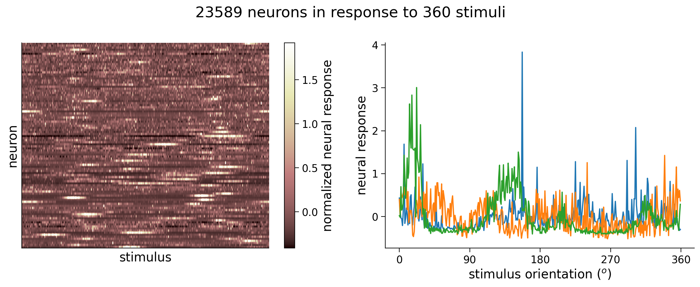
We will be exploring neural activity in mice while the mice is viewing oriented grating stimuli on a screen in front of it. We record neural activity using a technique called two-photon calcium imaging, which allows us to record many thousands of neurons simultanously. The neurons light up when they fire. We then convert this imaging data to a matrix of neural responses by stimuli presented. For the purposes of this tutorial we are going to bin the neural responses and compute each neuron’s tuning curve. We used bins of 1 degree. We will use the response of all neurons in a single bin to try to predict which stimulus was shown. So we are going to be using the responses of 24000 neurons to try to predict 360 different possible stimulus conditions corresponding to each degree of orientation - which means we’re in the regime of big data!

In the next cell, we have provided code to load the data and plot the matrix of neural responses.

Next to it, we plot the tuning curves of three randomly selected neurons. These tuning curves are the averaged response of each neuron to oriented stimuli within 1\(^\circ\), and since there are 360\(^\circ\) in total, we have 360 responses.

In the recording, there were actually thousands of stimuli shown, but in practice we often create these tuning curves because we want to visualize averaged responses with respect to the variable we varied in the experiment, in this case stimulus orientation.

Execute this cell to load and visualize data

../../../_images/f1a082ef66a3953f82d6b258817b34df94ab60cdacf785475276894d9c9e7a95.png

We will split our data into a training set and test set. In particular, we will have a training set of orientations (stimuli_train) and the corresponding responses (resp_train). Our testing set will have held-out orientations (stimuli_test) and the corresponding responses (resp_test).

Execute this cell to split into training and test sets

Section 2: Deep feed-forward networks in pytorch#

Click here for text recap of relevant part of video

We can build a linear network with no hidden layers, where the stimulus prediction \(y\) is a product of weights \(\mathbf{W}_{out}\) and neural responses \(\mathbf{r}\) with an added term \(\mathbf{b}\) which is called the bias term. When you fit a linear model such as this you minimize the squared error between the predicted stimulus \(y\) and the true stimulus \(\tilde{y}\), this is the “loss function”.

(224)#\[\begin{align} L &= (y - \tilde{y})^2 \\ &= ((\mathbf{W}^{out} \mathbf{r} + \mathbf{b}) - \tilde{y})^2 \end{align}\]

The solution to minimizing this loss function in a linear model can be found in closed form, and you learned how to solve this linear regression problem in the first week if you remember. If we use a simple linear model for this data we are able to predict the stimulus within 2-3 degrees. Let’s see if we can predict the neural activity better with a deep network.

Let’s add a hidden layer with \(M\) units to this linear model, where now the output \(y\) is as follows:

(225)#\[\begin{align} \mathbf{h} &= \mathbf{W}^{in} \mathbf{r} + \mathbf{b}^{in}, && [\mathbf{W}^{in}: M \times N \, , \, \mathbf{b}^{in}: M \times 1] \, , \\ y &= \mathbf{W}^{out} \mathbf{h} + \mathbf{b}^{out}, && [\mathbf{W}^{out}: 1 \times M\, , \, \mathbf{b}^{in}: 1 \times 1] \, , \end{align}\]

Note this linear network with one hidden layer where \(M\) hidden units is less than \(N\) inputs is equivalent to performing reduced rank regression, a technique that is useful for regularizing your regression model.

Adding this hidden layer means the model now has a depth of \(1\). The number of units \(M\) is termed the width of the network. Increasing the depth and the width of the network can increase the expressivity of the model – in other words how well it can fit complex non-linear functions. Many state-of-the-art models now have close to 100 layers! But for now let’s start with a model with a depth of \(1\) and see if we can improve our prediction of the stimulus. See bonus section 1 for a deeper discussion of what this choice entails, and when one might want to use deeper/shallower and wider/narrower architectures.

The \(M\)-dimensional vector \(\mathbf{h}\) denotes the activations of the hidden layer of the network. The blue components of this diagram denote the parameters of the network, which we will later optimize with gradient descent. These include all the weights and biases \(\mathbf{W}^{in}, \mathbf{b}^{in}, \mathbf{W}^{out}, \mathbf{b}^{out}\). The weights are matrices of size (# of outputs, # of inputs) that are multiplied by the input of each layer, like the regression coefficients in linear regression. The biases are vectors of size (# of outputs, 1), like the intercept term in linear regression (see W1D3 for more details on multivariate linear regression).

We’ll now build a simple deep neural network that takes as input a vector of neural responses and outputs a single number representing the decoded stimulus orientation.

Let \(\mathbf{r}^{(n)} = \begin{bmatrix} r_1^{(n)} & r_2^{(n)} & \ldots & r_N^{(n)} \end{bmatrix}^\top\) denote the vector of neural responses (of neurons \(1, \ldots, N\)) to the \(n\)th stimulus. The network we will use is described by the following set of equations:

(226)#\[\begin{align} \mathbf{h}^{(n)} &= \mathbf{W}^{in} \mathbf{r}^{(n)} + \mathbf{b}^{in}, && [\mathbf{W}^{in}: M \times N \, , \, \mathbf{b}^{in}: M \times 1] \, , \\ y^{(n)} &= \mathbf{W}^{out} \mathbf{h}^{(n)} + \mathbf{b}^{out}, && [\mathbf{W}^{out}: 1 \times M \, , \, \mathbf{b}^{in}: 1 \times 1] \, , \end{align}\]

where \(y^{(n)}\) denotes the scalar output of the network: the decoded orientation of the \(n\)-th stimulus.

Section 2.1: Introduction to PyTorch#

Estimated timing to here from start of tutorial: 16 min

Here, we’ll use the PyTorch package to build, run, and train deep networks of this form in Python. PyTorch uses a data type called a torch.Tensor. They are effectively just like numpy arrays, except that they have some important attributes and methods needed for automatic differentiation (to be discussed below). They also come along with infrastructure for easily storing and computing with them on GPU’s, a capability we won’t touch on here but which can be really useful in practice.

Click here for text recap of relevant part of video

First we import the pytorch library called torch and its neural network module nn. Next we will create a class for the deep network called DeepNet. A class has functions which are called methods. A class in python is initialized using a method called __init__. In this case the init method is declared to takes two inputs (other than the self input which represents the class itself), which are n_inputs and n_hidden. In our case n_inputs is the number of neurons we are using to do the prediction, and n_hidden is the number of hidden units. We first call the super function to invoke the nn.Module’s init function. Next we add the hidden layer in_layer as an attribute of the class. It is a linear layer called nn.Linear with size n_inputs by n_hidden. Then we add a second linear layer out_layer of size n_hidden by 1, because we are predicting one output - the orientation of the stimulus. PyTorch will initialize all weights and biases randomly.

Note the number of hidden units n_hidden is a parameter that we are free to vary in deciding how to build our network. See Bonus Section 1 for a discussion of how this architectural choice affects the computations the network can perform.

Next we add another method to the class called forward. This is the method that runs when you call the class as a function. It takes as input r which is the neural responses. Then r is sent through the linear layers in_layer and out_layer and returns our prediction y. Let’s create an instantiation of this class called net with 200 hidden units with net = DeepNet(n_neurons, 200). Now we can run the neural response through the network to predict the stimulus (net(r)); running the “net” this way calls the forward method.

The next cell contains code for building the deep network we defined above and in the video using the nn.Module base class for deep neural network models (documentation here).

class DeepNet(nn.Module):
  """Deep Network with one hidden layer

  Args:
    n_inputs (int): number of input units
    n_hidden (int): number of units in hidden layer

  Attributes:
    in_layer (nn.Linear): weights and biases of input layer
    out_layer (nn.Linear): weights and biases of output layer

  """

  def __init__(self, n_inputs, n_hidden):
    super().__init__()  # needed to invoke the properties of the parent class nn.Module
    self.in_layer = nn.Linear(n_inputs, n_hidden) # neural activity --> hidden units
    self.out_layer = nn.Linear(n_hidden, 1) # hidden units --> output

  def forward(self, r):
    """Decode stimulus orientation from neural responses

    Args:
      r (torch.Tensor): vector of neural responses to decode, must be of
        length n_inputs. Can also be a tensor of shape n_stimuli x n_inputs,
        containing n_stimuli vectors of neural responses

    Returns:
      torch.Tensor: network outputs for each input provided in r. If
        r is a vector, then y is a 1D tensor of length 1. If r is a 2D
        tensor then y is a 2D tensor of shape n_stimuli x 1.

    """
    h = self.in_layer(r)  # hidden representation
    y = self.out_layer(h)
    return y

Section 2.2: Activation functions#

Estimated timing to here from start of tutorial: 25 min

Video 2: Nonlinear activation functions#

Submit your feedback#

This video covers adding a nonlinear activation function, specifically a Rectified Linear Unit (ReLU), to the linear network.

Click here for text recap of video

Note that the deep network we constructed above comprises solely linear operations on each layer: each layer is just a weighted sum of all the elements in the previous layer. It turns out that linear hidden layers like this aren’t particularly useful, since a sequence of linear transformations is actually essentially the same as a single linear transformation. We can see this from the above equations by plugging in the first one into the second one to obtain

(227)#\[\begin{equation} y^{(n)} = \mathbf{W}^{out} \left( \mathbf{W}^{in} \mathbf{r}^{(n)} + \mathbf{b}^{in} \right) + \mathbf{b}^{out} = \mathbf{W}^{out}\mathbf{W}^{in} \mathbf{r}^{(n)} + \left( \mathbf{W}^{out}\mathbf{b}^{in} + \mathbf{b}^{out} \right) \end{equation}\]

In other words, the output is still just a weighted sum of elements in the input – the hidden layer has done nothing to change this.

To extend the set of computable input/output transformations to more than just weighted sums, we’ll incorporate a non-linear activation function in the hidden units. This is done by simply modifying the equation for the hidden layer activations to be

(228)#\[\begin{equation} \mathbf{h}^{(n)} = \phi(\mathbf{W}^{in} \mathbf{r}^{(n)} + \mathbf{b}^{in}) \end{equation}\]

where \(\phi\) is referred to as the activation function. Using a non-linear activation function will ensure that the hidden layer performs a non-linear transformation of the input, which will make our network much more powerful (or expressive, see Bonus Section 1). In practice, deep networks always use non-linear activation functions.

The most common non-linearity used is the rectified linear unit (or ReLU), which is a max(0, x) function. At the beginning of neural network development, researchers experimented with different non-linearities such as sigmoid and tanh functions, but in the end they found that RELU activation functions worked the best. It works well because the gradient is able to back-propagate through the network as long as the input is positive - the gradient is 1 for all values of x greater than 0. If you use a saturating non-linearity then the gradients will be very small in the saturating regimes, reducing the effective computing regime of the unit.

Coding Exercise 2.2: Nonlinear Activations#

Create a new class DeepNetReLU by modifying our above deep network model to add a non-linear activation function \(\phi\):

(229)#\[\begin{equation} \mathbf{h}^{(n)} = \phi(\mathbf{W}^{in} \mathbf{r}^{(n)} + \mathbf{b}^{in}) \end{equation}\]

We’ll use the linear rectification function:

(230)#\[\begin{equation} \phi(x) = \begin{cases} x & \text{if } x > 0 \\ 0 & \text{else} \end{cases} \end{equation}\]

which can be implemented in PyTorch using torch.relu(). Hidden layers with this activation function are typically referred to as “Rectified Linear Units”, or ReLU’s.

Initialize this network with 10 hidden units and run on an example stimulus.

Hint: you only need to modify the forward() method of the above DeepNet() class to include torch.relu().

We then initialize and run this network. We use it to decode stimulus orientation (true stimulus given by ori) from a vector of neural responses r to the very first stimulus. Note that when the initialized network class is called as a function on an input (e.g., net(r)), its .forward() method is called. This is a special property of the nn.Module class.

Note that the decoded orientations at this point will be nonsense, since the network has been initialized with random weights. Below, we’ll learn how to optimize these weights for good stimulus decoding.

class DeepNetReLU(nn.Module):
  """ network with a single hidden layer h with a RELU """

  def __init__(self, n_inputs, n_hidden):
    super().__init__()  # needed to invoke the properties of the parent class nn.Module
    self.in_layer = nn.Linear(n_inputs, n_hidden) # neural activity --> hidden units
    self.out_layer = nn.Linear(n_hidden, 1) # hidden units --> output

  def forward(self, r):

    ############################################################################
    ## TO DO for students: write code for computing network output using a
    ## rectified linear activation function for the hidden units
    # Fill out function and remove
    raise NotImplementedError("Student exercise: complete DeepNetReLU forward")
    ############################################################################

    h = ... # h is size (n_inputs, n_hidden)
    y = ... # y is size (n_inputs, 1)


    return y


# Set random seeds for reproducibility
np.random.seed(1)
torch.manual_seed(1)

# Initialize a deep network with M=200 hidden units
net = DeepNetReLU(n_neurons, 200)

# Get neural responses (r) to and orientation (ori) to one stimulus in dataset
r, ori = get_data(1, resp_train, stimuli_train)  # using helper function get_data

# Decode orientation from these neural responses using initialized network
out = net(r)  # compute output from network, equivalent to net.forward(r)

print(f'decoded orientation: {out.item():.2f} degrees')
print(f'true orientation: {ori.item():.2f} degrees')

The decoded orientation is 0.17 \(^{\circ}\) while the true orientation is 139.00 \(^{\circ}\). You should see:

decoded orientation: 0.17 degrees
true orientation: 139.00 degrees

Click for solution

Submit your feedback#

Section 3: Loss functions and gradient descent#

Video 3: Loss functions & gradient descent#

Submit your feedback#

This video covers loss functions, gradient descent, and how to implement these in Pytorch.

Section 3.1: Loss functions#

Estimated timing to here from start of tutorial: 40 min

Because the weights of the network are currently randomly chosen, the outputs of the network are nonsense: the decoded stimulus orientation is nowhere close to the true stimulus orientation. We’ll shortly write some code to change these weights so that the network does a better job of decoding.

But to do so, we first need to define what we mean by “better”. One simple way of defining this is to use the squared error

(231)#\[\begin{equation} L = (y - \tilde{y})^2 \end{equation}\]

where \(y\) is the network output and \(\tilde{y}\) is the true stimulus orientation. When the decoded stimulus orientation is far from the true stimulus orientation, \(L\) will be large. We thus refer to \(L\) as the loss function, as it quantifies how bad the network is at decoding stimulus orientation.

Click here for text recap of relevant part of video

First we run the neural responses through the network net to get the output out. Then we declare our loss function, we will use the built in nn.MSELoss function for this purpose: loss_fn = nn.MSELoss(). This loss function takes two inputs, the network output out and the true stimulus orientations ori and finds the mean squared error: loss = loss_fn(out, ori). Specifically, it will take as arguments a batch of network outputs \(y_1, y_2, \ldots, y_P\) and corresponding target outputs \(\tilde{y}_1, \tilde{y}_2, \ldots, \tilde{y}_P\), and compute the mean squared error (MSE)

(232)#\[\begin{equation} L = \frac{1}{P}\sum_{n=1}^P \left(y^{(n)} - \tilde{y}^{(n)}\right)^2 \end{equation}\]

where \(P\) is the number of different stimuli in a batch, called the batch size.

Computing MSE

Evaluate the mean squared error for a deep network with \(M=10\) rectified linear units, on the decoded orientations from neural responses to 20 random stimuli.

# Set random seeds for reproducibility
np.random.seed(1)
torch.manual_seed(1)

# Initialize a deep network with M=10 hidden units
net = DeepNetReLU(n_neurons, 10)

# Get neural responses to first 20 stimuli in the data set
r, ori = get_data(20, resp_train, stimuli_train)

# Decode orientation from these neural responses
out = net(r)

# Initialize PyTorch mean squared error loss function (Hint: look at nn.MSELoss)
loss_fn = nn.MSELoss()

# Evaluate mean squared error
loss = loss_fn(out, ori)

print(f'mean squared error: {loss:.2f}')

You should see a mean squared error of 42949.14.

Section 3.2: Optimization with gradient descent#

Estimated timing to here from start of tutorial: 50 min

Click here for text recap of relevant part of video

Next we minimize this loss function using gradient descent. In gradient descent we compute the gradient of the loss function with respect to each parameter (all \(W\)’s and \(b\)’s). We then update the parameters by subtracting the learning rate times the gradient.

Let’s visualize this loss function \(L\) with respect to a weight \(w\). If the gradient is positive (the slope \(\frac{dL}{dw}\) > 0) as in this case then we want to move in the opposite direction which is negative. So we update the \(w\) accordingly in the negative direction on each iteration. Once the iterations complete the weight will ideally be at a value that minimizes the cost function.

In reality these cost functions are not convex like this one and depend on hundreds of thousands of parameters. There are tricks to help navigate this rocky cost landscape such as adding momentum or changing the optimizer but we won’t have time to get into that today. There are also ways to change the architecture of the network to improve optimization, such as including skip connections. These skip connections are used in residual networks and allow for the optimization of many layer networks.

Execute this cell to view gradient descent gif

We’ll use the gradient descent (GD) algorithm to modify our weights to reduce the loss function, which consists of iterating three steps.

Evaluate the loss on the training data,

out = net(train_data)
loss = loss_fn(out, train_labels)

where train_data are the network inputs in the training data (in our case, neural responses), and train_labels are the target outputs for each input (in our case, true stimulus orientations). 2. Compute the gradient of the loss with respect to each of the network weights. In PyTorch, we can do this with the .backward() method of the loss loss. Note that the gradients of each parameter need to be cleared before calling .backward(), or else PyTorch will try to accumulate gradients across iterations. This can again be done using built-in optimizers via the method .zero_grad(). Putting these together we have

optimizer.zero_grad()
loss.backward()

Update the network weights by descending the gradient. In Pytorch, we can do this using built-in optimizers. We’ll use the optim.SGD optimizer (documentation here) which updates parameters along the negative gradient, scaled by a learning rate. To initialize this optimizer, we have to tell it

which parameters to update, and
what learning rate to use

For example, to optimize all the parameters of a network net using a learning rate of .001, the optimizer would be initialized as follows

optimizer = optim.SGD(net.parameters(), lr=.001)

where .parameters() is a method of the nn.Module class that returns a Python generator object over all the parameters of that nn.Module class (in our case, \(\mathbf{W}^{in}, \mathbf{b}^{in}, \mathbf{W}^{out}, \mathbf{b}^{out}\)).

After computing all the parameter gradients in step 2, we can then update each of these parameters using the .step() method of this optimizer,

optimizer.step()

In the next exercise, we’ll give you a code skeleton for implementing the GD algorithm. Your job will be to fill in the blanks.

For the mathematical details of the GD algorithm, see bonus section 2.1.

In this case we are using gradient descent (not stochastic gradient descent) because we are computing the gradient over ALL training data at once. Normally there is too much training data to do this in practice, and for instance the neural responses may be divided into sets of 20 stimuli. An epoch in deep learning is defined as the forward and backward pass of all the training data through the network. We will run the forward and backward pass of the network here for 20 epochs, in practice training may require thousands of epochs.

See bonus section 2.2 for a more detailed discussion of stochastic gradient descent.

Coding Exercise 3.2: Gradient descent in PyTorch#

Complete the function train() that uses the gradient descent algorithm to optimize the weights of a given network. This function takes as input arguments

net: the PyTorch network whose weights to optimize
loss_fn: the PyTorch loss function to use to evaluate the loss
train_data: the training data to evaluate the loss on (i.e., neural responses to decode)
train_labels: the target outputs for each data point in train_data (i.e., true stimulus orientations)

We will then train a neural network on our data and plot the loss (mean squared error) over time. When we run this function, behind the scenes PyTorch is actually changing the parameters inside this network to make the network better at decoding, so its weights will now be different than they were at initialization.

def train(net, loss_fn, train_data, train_labels,
          n_epochs=50, learning_rate=1e-4):
  """Run gradient descent to optimize parameters of a given network

  Args:
    net (nn.Module): PyTorch network whose parameters to optimize
    loss_fn: built-in PyTorch loss function to minimize
    train_data (torch.Tensor): n_train x n_neurons tensor with neural
      responses to train on
    train_labels (torch.Tensor): n_train x 1 tensor with orientations of the
      stimuli corresponding to each row of train_data
    n_epochs (int, optional): number of epochs of gradient descent to run
    learning_rate (float, optional): learning rate to use for gradient descent

  Returns:
    (list): training loss over iterations

  """

  # Initialize PyTorch SGD optimizer
  optimizer = optim.SGD(net.parameters(), lr=learning_rate)

  # Placeholder to save the loss at each iteration
  train_loss = []

  # Loop over epochs
  for i in range(n_epochs):

    ######################################################################
    ## TO DO for students: fill in missing code for GD iteration
    raise NotImplementedError("Student exercise: write code for GD iterations")
    ######################################################################

    # compute network output from inputs in train_data
    out = ...  # compute network output from inputs in train_data

    # evaluate loss function
    loss = loss_fn(out, train_labels)

    # Clear previous gradients
    ...

    # Compute gradients
    ...

    # Update weights
    ...

    # Store current value of loss
    train_loss.append(loss.item())  # .item() needed to transform the tensor output of loss_fn to a scalar

    # Track progress
    if (i + 1) % (n_epochs // 5) == 0:
      print(f'iteration {i + 1}/{n_epochs} | loss: {loss.item():.3f}')

  return train_loss


# Set random seeds for reproducibility
np.random.seed(1)
torch.manual_seed(1)

# Initialize network with 10 hidden units
net = DeepNetReLU(n_neurons, 10)

# Initialize built-in PyTorch MSE loss function
loss_fn = nn.MSELoss()

# Run gradient descent on data
train_loss = train(net, loss_fn, resp_train, stimuli_train)

# Plot the training loss over iterations of GD
plot_train_loss(train_loss)

Click for solution

Example output:

Submit your feedback#

We can further improve our model - please see the Bonus part of the Tutorial when you have time to dive deeper into this model by evaluating and improving its performance by visualizing the weights, looking at performance on test data, switching to a new loss function and adding regularization.

Summary#

Estimated timing of tutorial: 1 hour, 20 minutes

We have now covered a number of common and powerful techniques for applying deep learning to decoding from neural data, some of which are common to almost any machine learning problem:

Building and training deep networks using the PyTorch nn.Module class and built-in optimizers
Choosing loss functions

An important aspect of this tutorial was the train() function we wrote in coding exercise 3.2. Note that it can be used to train any network to minimize any loss function on any training data. This is the power of using PyTorch to train neural networks and, for that matter, any other model! There is nothing in the nn.Module class that forces us to use nn.Linear layers that implement neural network operations. You can actually put anything you want inside the .__init__() and .forward() methods of this class. As long as its parameters and computations involve only torch.Tensor’s, and the model is differentiable, you’ll then be able to optimize the parameters of this model in exactly the same way we optimized the deep networks here.

What kinds of conclusions can we draw from these sorts of analyses? If we can decode the stimulus well from visual cortex activity, that means that there is information about this stimulus available in the visual cortex. Whether or not the animal uses that information to make decisions is not determined from an analysis like this. In fact mice perform poorly in orientation discrimination tasks compared to monkeys and humans, even though they have information about these stimuli in their visual cortex. Why do you think they perform poorly in orientation discrimination tasks?

See Stringer, et al., 2021 for some potential hypotheses, but this is totally an open question!

Bonus#

Bonus Section 1: Neural network depth, width and expressivity#

Two important architectural choices that always have to be made when constructing deep feed-forward networks like those used here are

the number of hidden layers, or the network’s depth
the number of units in each layer, or the layer widths

Here, we restricted ourselves to networks with a single hidden layer with a width of \(M\) units, but it is easy to see how this code could be adapted to arbitrary depths. Adding another hidden layer simply requires adding another nn.Linear module to the __init__() method and incorporating it into the .forward() method.

The depth and width of a network determine the set of input/output transformations that it can perform, often referred to as its expressivity. The deeper and wider the network, the more expressive it is; that is, the larger the class of input/output transformations it can compute. In fact, it turns out that an infinitely wide or infinitely deep networks can in principle compute (almost) any input/output transformation.

A classic mathematical demonstration of the power of depth is given by the so-called XOR problem. This toy problem demonstrates how even a single hidden layer can drastically expand the set of input/output transformations a network can perform, relative to a shallow network with no hidden layers. The key intuition is that the hidden layer allows you to represent the input in a new format, which can then allow you to do almost anything you want with it. The wider this hidden layer, the more flexibility you have in this representation. In particular, if you have more hidden units than input units, then the hidden layer representation of the input is higher-dimensional than the raw data representation. This higher dimensionality effectively gives you more “room” to perform arbitrary computations in. It turns out that even with just this one hidden layer, if you make it wide enough you can actually approximate any input/output transformation you want. See here for a neat visual demonstration of this.

In practice, however, it turns out that increasing depth seems to grant more expressivity with fewer units than increasing width does (for reasons that are not well understood). It is for this reason that truly deep networks are almost always used in machine learning, which is why this set of techniques is often referred to as deep learning.

That said, there is a cost to making networks deeper and wider. The bigger your network, the more parameters (i.e., weights and biases) it has, which need to be optimized! The extra expressivity afforded by higher width and/or depth thus carries with it (at least) two problems:

optimizing more parameters usually requires more data
a more highly parameterized network is more prone to overfit to the training data, so requires more sophisticated optimization algorithms to ensure generalization

Bonus Section 2: Gradient descent#

Bonus Section 2.1: Gradient descent equations#

Here we provide the equations for the three steps of the gradient descent algorithm, as applied to our decoding problem:

Evaluate the loss on the training data. For a mean squared error loss, this is given by

(233)#\[\begin{equation} L = \frac{1}{P}\sum_{n=1}^P \left( y^{(n)} - \tilde{y}^{(n)} \right)^2 \end{equation}\]

where \(y^{(n)}\) denotes the stimulus orientation decoded from the population response \(\mathbf{r}^{(n)}\) to the \(n\)th stimulus in the training data, and \(\tilde{y}^{(n)}\) is the true orientation of that stimulus. \(P\) denotes the total number of data samples in the training set. In the syntax of our train() function above, \(\mathbf{r}^{(n)}\) is given by train_data[n, :] and \(\tilde{y}^{(n)}\) by train_labels[n].

Compute the gradient of the loss with respect to each of the network weights. In our case, this entails computing the quantities

(234)#\[\begin{equation} \frac{\partial L}{\partial \mathbf{W}^{in}}, \frac{\partial L}{\partial \mathbf{b}^{in}}, \frac{\partial L}{\partial \mathbf{W}^{out}}, \frac{\partial L}{\partial \mathbf{b}^{out}} \end{equation}\]

Usually, we would require lots of math in order to derive each of these gradients, and lots of code to compute them. But this is where PyTorch comes to the rescue! Using a cool technique called automatic differentiation, PyTorch automatically calculates these gradients when the .backward() function is called.

More specifically, when this function is called on a particular variable (e.g., loss, as above), PyTorch will compute the gradients with respect to each network parameter. These are computed and stored behind the scenes, and can be accessed through the .grad attribute of each of the network’s parameters. As we saw above, however, we actually never need to look at or call these gradients when implementing gradient descent, as this can be taken care of by PyTorch’s built-in optimizers, like optim.SGD.

Update the network weights by descending the gradient:

(235)#\[\begin{align} \mathbf{W}^{in} &\leftarrow \mathbf{W}^{in} - \alpha \frac{\partial L}{\partial \mathbf{W}^{in}} \\ \mathbf{b}^{in} &\leftarrow \mathbf{b}^{in} - \alpha \frac{\partial L}{\partial \mathbf{b}^{in}} \\ \mathbf{W}^{out} &\leftarrow \mathbf{W}^{out} - \alpha \frac{\partial L}{\partial \mathbf{W}^{out}} \\ \mathbf{b}^{out} &\leftarrow \mathbf{b}^{out} - \alpha \frac{\partial L}{\partial \mathbf{b}^{out}} \end{align}\]

where \(\alpha\) is called the learning rate. This hyperparameter of the SGD algorithm controls how far we descend the gradient on each iteration. It should be as large as possible so that fewer iterations are needed, but not too large so as to avoid parameter updates from skipping over minima in the loss landscape.

While the equations written down here are specific to the network and loss function considered in this tutorial, the code provided above for implementing these three steps is completely general: no matter what loss function or network you are using, exactly the same commands can be used to implement these three steps.

The way that the gradients are calculated is called backpropagation. We have a loss function:

(236)#\[\begin{align} L &= (y - \tilde{y})^2 \\ &= (\mathbf{W}^{out} \mathbf{h} - \tilde{y})^2 \end{align}\]

where \(\mathbf{h} = \phi(\mathbf{W}^{in} \mathbf{r} + \mathbf{b}^{in})\), and \(\phi(\cdot)\) is the activation function, e.g., RELU. You may see that \(\frac{\partial L}{\partial \mathbf{W}^{out}}\) is simple to calculate as it is on the outside of the equation (it is also a vector in this case, not a matrix, so the derivative is standard):

(237)#\[\begin{equation} \frac{\partial L}{\partial \mathbf{W}^{out}} = 2 (\mathbf{W}^{out} \mathbf{h} - \tilde{y})\mathbf{h}^\top \end{equation}\]

Now let’s compute the derivative with respect to \(\mathbf{W}^{in}\) using the chain rule. Note it is only positive if the output is positive due to the RELU activation function \(\phi\). For the chain rule we need the derivative of the loss with respect to \(\mathbf{h}\):

(238)#\[\begin{equation} \frac{\partial L}{\partial \mathbf{h}} = 2 \mathbf{W}^{out \top} (\mathbf{W}^{out} \mathbf{h} - \tilde{y}) \end{equation}\]

Thus,

(239)#\[\begin{align} \frac{\partial L}{\partial \mathbf{W}^{in}} &= \begin{cases} \frac{\partial L}{\partial \mathbf{h}} \frac{\partial \mathbf{h}}{\partial \mathbf{W}^{in}} & \text{if } \mathbf{h} > 0 \\ 0 & \text{otherwise} \end{cases} \\ &= \begin{cases} 2 \mathbf{W}^{out \top} (\mathbf{W}^{out} \mathbf{h} - \tilde{y}) \mathbf{r}^\top & \text{if } \mathbf{h} > 0 \\ 0 & \text{otherwise} \end{cases} \end{align}\]

Notice that:

(240)#\[\begin{equation} \frac{\partial \mathbf{h}}{\partial \mathbf{W}^{in}}=\mathbf{r}^\top \odot \phi^\prime \end{equation}\]

where \(\odot\) denotes the Hadamard product (i.e., elementwise multiplication) and \(\phi^\prime\) is the derivative of the activation function. In case of RELU:

(241)#\[\begin{align} \phi^\prime &= \begin{cases} 1 & \text{if } \mathbf{h} > 0 \\ 0 & \text{otherwise} \end{cases} \end{align}\]

It is most efficient to compute the derivative once for the last layer, then once for the next layer and multiply by the previous layer’s derivative and so on using the chain rule. Each of these operations is relatively fast, making training of deep networks feasible.

The command loss.backward() computes these gradients for the defined loss with respect to each network parameter. The computation is done using automatic differentiation, which implements backpropagation. Note that this works no matter how big/small the network is, allowing us to perform gradient descent for any deep network model built using PyTorch.

Bonus Section 2.2: Stochastic gradient descent (SGD) vs. gradient descent (GD)#

In this tutorial, we used the gradient descent algorithm, which differs in a subtle yet very important way from the more commonly used stochastic gradient descent (SGD) algorithm. The key difference is in the very first step of each iteration, where in the GD algorithm we evaluate the loss at every data sample in the training set. In SGD, on the other hand, we evaluate the loss only at a random subset of data samples from the full training set, called a mini-batch. At each iteration, we randomly sample a mini-batch to perform steps 1-3 on. All the above equations still hold, but now the \(P\) data samples \(\mathbf{r}^{(n)}, \tilde{y}^{(n)}\) denote a mini-batch of \(P\) random samples from the training set, rather than the whole training set.

There are several reasons why one might want to use SGD instead of GD. The first is that the training set might be too big, so that we actually can’t actually evaluate the loss on every single data sample in it. In this case, GD is simply infeasible, so we have no choice but to turn to SGD, which bypasses the restrictive memory demands of GD by subsampling the training set into smaller mini-batches.

But, even when GD is feasible, SGD turns out to often be better. The stochasticity induced by the extra random sampling step in SGD effectively adds some noise in the search for local minima of the loss function. This can be really useful for avoiding potential local minima, and enforce that whatever minimum is converged to is a good one. This is particularly important when networks are wider and/or deeper, in which case the large number of parameters can lead to overfitting.

Here, we used only GD because (1) it is simpler, and (2) it suffices for the problem being considered here. Because we have so many neurons in our data set, decoding is not too challenging and doesn’t require a particularly deep or wide network. The small number of parameters in our deep networks therefore can be optimized without a problem using GD.

Tutorial 1: Decoding Neural Responses

Contents

Tutorial 1: Decoding Neural Responses#

Tutorial Objectives#

Setup#

Install and import feedback gadget#

Figure Settings#

Plotting Functions#

Helper Functions#

Data retrieval and loading#

Section 0: Decoding Task#

Video 1: Decoding from neural data using feed-forward networks in pytorch#

Submit your feedback#

Section 1: Load, split and visualize data#

Section 2: Deep feed-forward networks in pytorch#

Section 2.1: Introduction to PyTorch#

Section 2.2: Activation functions#

Video 2: Nonlinear activation functions#

Submit your feedback#

Coding Exercise 2.2: Nonlinear Activations#

Submit your feedback#

Section 3: Loss functions and gradient descent#

Video 3: Loss functions & gradient descent#

Submit your feedback#

Section 3.1: Loss functions#

Section 3.2: Optimization with gradient descent#

Coding Exercise 3.2: Gradient descent in PyTorch#

Submit your feedback#

Summary#

Bonus#

Bonus Section 1: Neural network depth, width and expressivity#

Bonus Section 2: Gradient descent#

Bonus Section 2.1: Gradient descent equations#

Bonus Section 2.2: Stochastic gradient descent (SGD) vs. gradient descent (GD)#