Tutorial 3: Synaptic transmission - Models of static and dynamic synapses

Tutorial 3: Synaptic transmission - Models of static and dynamic synapses#

Week 2, Day 3: Biological Neuron Models

By Neuromatch Academy

Content creators: Qinglong Gu, Songtin Li, John Murray, Richard Naud, Arvind Kumar

Content reviewers: Maryam Vaziri-Pashkam, Ella Batty, Lorenzo Fontolan, Richard Gao, Matthew Krause, Spiros Chavlis, Michael Waskom

Post-Production team: Gagana B, Spiros Chavlis

Tutorial Objectives#

Estimated timing of tutorial: 1 hour, 10 min

Synapses connect neurons into neural networks or circuits. Specialized electrical synapses make direct, physical connections between neurons. In this tutorial, however, we will focus on chemical synapses, which are more common in the brain. These synapses do not physically join neurons. Instead, a spike in the presynaptic cell causes a chemical, or neurotransmitter, to be released into a small space between the neurons called the synaptic cleft. Once the chemical diffuses across that space, it changes the permeability of the postsynaptic membrane, which may result in a positive or negative change in the membrane voltage.

In this tutorial, we will model chemical synaptic transmission and study some interesting effects produced by static synapses and dynamic synapses.

First, we will start by writing code to simulate static synapses – whose weight is always fixed. Next, we will extend the model and model dynamic synapses – whose synaptic strength is dependent on the recent spike history: synapses can either progressively increase or decrease the size of their effects on the post-synaptic neuron, based on the recent firing rate of its presynaptic partners. This feature of synapses in the brain is called Short-Term Plasticity and causes synapses to undergo Facilitation or Depression.

Our goals for this tutorial are to:

simulate static synapses and study how excitation and inhibition affect the patterns in the neurons’ spiking output
define mean- or fluctuation-driven regimes
simulate short-term dynamics of synapses (facilitation and depression)
study how a change in pre-synaptic firing history affects the synaptic weights (i.e., PSP amplitude)

Setup#

Install and import feedback gadget#

# Imports
import matplotlib.pyplot as plt
import numpy as np

Figure Settings#

Plotting Functions#

Show code cell source Hide code cell source

# @title Plotting Functions

def my_illus_LIFSYN(pars, v_fmp, v):
  """
  Illustartion of FMP and membrane voltage

  Args:
    pars  : parameters dictionary
    v_fmp : free membrane potential, mV
    v     : membrane voltage, mV

  Returns:
    plot of membrane voltage and FMP, alongside with the spiking threshold
    and the mean FMP (dashed lines)
  """

  plt.figure(figsize=(14, 5))
  plt.plot(pars['range_t'], v_fmp, 'r', lw=1.,
           label='Free mem. pot.', zorder=2)
  plt.plot(pars['range_t'], v, 'b', lw=1.,
           label='True mem. pot', zorder=1, alpha=0.7)
  plt.axhline(pars['V_th'], 0, 1, color='k', lw=2., ls='--',
              label='Spike Threshold', zorder=1)
  plt.axhline(np.mean(v_fmp), 0, 1, color='r', lw=2., ls='--',
              label='Mean Free Mem. Pot.', zorder=1)
  plt.xlabel('Time (ms)')
  plt.ylabel('V (mV)')
  plt.legend(loc=[1.02, 0.68])
  plt.show()


def plot_volt_trace(pars, v, sp, show=True):
  """
  Plot trajetory of membrane potential for a single neuron

  Args:
    pars   : parameter dictionary
    v      : volt trajetory
    sp     : spike train

  Returns:
    figure of the membrane potential trajetory for a single neuron
  """

  V_th = pars['V_th']
  dt = pars['dt']
  if sp.size:
    sp_num = (sp/dt).astype(int) - 1
    v[sp_num] += 10

  plt.plot(pars['range_t'], v, 'b')
  plt.axhline(V_th, 0, 1, color='k', ls='--', lw=1.)
  plt.xlabel('Time (ms)')
  plt.ylabel('V (mV)')
  if show:
    plt.show()


def my_illus_STD(Poisson=False, rate=20., U0=0.5,
                 tau_d=100., tau_f=50., plot_out=True):
  """
   Only for one presynaptic train

  Args:
    Poisson    : Poisson or regular input spiking trains
    rate       : Rate of input spikes, Hz
    U0         : synaptic release probability at rest
    tau_d      : synaptic depression time constant of x [ms]
    tau_f      : synaptic facilitation time constantr of u [ms]
    plot_out   : whether ot not to plot, True or False

  Returns:
    Nothing.
  """

  T_simu = 10.0 * 1000 / (1.0 * rate)  # 10 spikes in the time window
  pars = default_pars(T=T_simu)
  dt = pars['dt']

  if Poisson:
    # Poisson type spike train
    pre_spike_train = Poisson_generator(pars, rate, n=1)
    pre_spike_train = pre_spike_train.sum(axis=0)
  else:
    # Regular firing rate
    isi_num = int((1e3/rate)/dt)  # number of dt
    pre_spike_train = np.zeros(len(pars['range_t']))
    pre_spike_train[::isi_num] = 1.

  u, R, g = dynamic_syn(g_bar=1.2, tau_syn=5., U0=U0,
                        tau_d=tau_d, tau_f=tau_f,
                        pre_spike_train=pre_spike_train,
                        dt=pars['dt'])

  if plot_out:
    plt.figure(figsize=(12, 6))

    plt.subplot(221)
    plt.plot(pars['range_t'], R, 'b', label='R')
    plt.plot(pars['range_t'], u, 'r', label='u')
    plt.legend(loc='best')
    plt.xlim((0, pars['T']))
    plt.ylabel(r'$R$ or $u$ (a.u)')
    plt.subplot(223)
    spT = pre_spike_train > 0
    t_sp = pars['range_t'][spT]  #spike times
    plt.plot(t_sp, 0. * np.ones(len(t_sp)), 'k|', ms=18, markeredgewidth=2)
    plt.xlabel('Time (ms)');
    plt.xlim((0, pars['T']))
    plt.yticks([])
    plt.title('Presynaptic spikes')

    plt.subplot(122)
    plt.plot(pars['range_t'], g, 'r', label='STP synapse')
    plt.xlabel('Time (ms)')
    plt.ylabel('g (nS)')
    plt.xlim((0, pars['T']))

    plt.tight_layout()
    plt.show()

  if not Poisson:
    return g[isi_num], g[9*isi_num]

Helper Functions#

Show code cell source Hide code cell source

# @title Helper Functions

def my_GWN(pars, mu, sig, myseed=False):
  """
  Args:
    pars       : parameter dictionary
    mu         : noise baseline (mean)
    sig        : noise amplitute (standard deviation)
    myseed     : random seed. int or boolean
                  the same seed will give the same random number sequence

  Returns:
    I          : Gaussian White Noise (GWN) input
  """

  # Retrieve simulation parameters
  dt, range_t = pars['dt'], pars['range_t']
  Lt = range_t.size

  # set random seed
  # you can fix the seed of the random number generator so that the results
  # are reliable. However, when you want to generate multiple realizations
  # make sure that you change the seed for each new realization.
  if myseed:
      np.random.seed(seed=myseed)
  else:
      np.random.seed()

  # generate GWN
  # we divide here by 1000 to convert units to seconds.
  I_GWN = mu + sig * np.random.randn(Lt) / np.sqrt(dt / 1000.)

  return I_GWN


def Poisson_generator(pars, rate, n, myseed=False):
  """
  Generates poisson trains

  Args:
    pars       : parameter dictionary
    rate       : noise amplitute [Hz]
    n          : number of Poisson trains
    myseed     : random seed. int or boolean

  Returns:
    pre_spike_train : spike train matrix, ith row represents whether
                      there is a spike in ith spike train over time
                      (1 if spike, 0 otherwise)
  """

  # Retrieve simulation parameters
  dt, range_t = pars['dt'], pars['range_t']
  Lt = range_t.size

  # set random seed
  if myseed:
      np.random.seed(seed=myseed)
  else:
      np.random.seed()

  # generate uniformly distributed random variables
  u_rand = np.random.rand(n, Lt)

  # generate Poisson train
  poisson_train = 1. * (u_rand < rate * (dt / 1000.))

  return poisson_train


def default_pars(**kwargs):
  pars = {}

  ### typical neuron parameters###
  pars['V_th'] = -55.    # spike threshold [mV]
  pars['V_reset'] = -75. # reset potential [mV]
  pars['tau_m'] = 10.    # membrane time constant [ms]
  pars['g_L'] = 10.      # leak conductance [nS]
  pars['V_init'] = -65.  # initial potential [mV]
  pars['E_L'] = -75.     # leak reversal potential [mV]
  pars['tref'] = 2.      # refractory time (ms)

  ### simulation parameters ###
  pars['T'] = 400.  # Total duration of simulation [ms]
  pars['dt'] = .1   # Simulation time step [ms]

  ### external parameters if any ###
  for k in kwargs:
    pars[k] = kwargs[k]

  pars['range_t'] = np.arange(0, pars['T'], pars['dt'])  # Vector of discretized time points [ms]

  return pars

In the Helper Function:

Gaussian white noise generator: my_GWN(pars, mu, sig, myseed=False)
Poissonian spike train generator: Poisson_generator(pars, rate, n, myseed=False)
default parameter function (as before)

Section 0: Static and Dynamic Synapses#

Video 1: Static and dynamic synapses#

Submit your feedback#

Section 1: Static synapses#

Estimated timing to here from start of tutorial: 20 min

Section 1.1: Simulate synaptic conductance dynamics#

Synaptic input in vivo consists of a mixture of excitatory neurotransmitters, which depolarizes the cell and drives it towards spike threshold, and inhibitory neurotransmitters that hyperpolarize it, driving it away from spike threshold. These chemicals cause specific ion channels on the postsynaptic neuron to open, resulting in a change in that neuron’s conductance and, therefore, the flow of current in or out of the cell.

This process can be modeled by assuming that the presynaptic neuron’s spiking activity produces transient changes in the postsynaptic neuron’s conductance (\(g_{\rm syn}(t)\)). Typically, the conductance transient is modeled as an exponential function.

Such conductance transients can be generated using a simple ordinary differential equation (ODE):

(293)#\[\begin{equation} \frac{dg_{\rm syn}(t)}{dt} = \bar{g}_{\rm syn} \sum_k \delta(t-t_k) -g_{\rm syn}(t)/\tau_{\rm syn} \end{equation}\]

where \(\bar{g}_{\rm syn}\) (often referred to as synaptic weight) is the maximum conductance elicited by each incoming spike, and \(\tau_{\rm syn}\) is the synaptic time constant. Note that the summation runs over all spikes received by the neuron at time \(t_k\).

Ohm’s law allows us to convert conductance changes to the current as:

(294)#\[\begin{equation} I_{\rm syn}(t) = g_{\rm syn}(t)(V(t)-E_{\rm syn}) \\ \end{equation}\]

The reversal potential \(E_{\rm syn}\) determines the direction of current flow and the excitatory or inhibitory nature of the synapse.

Thus, incoming spikes are filtered by an exponential-shaped kernel, effectively low-pass filtering the input. In other words, synaptic input is not white noise, but it is, in fact, colored noise, where the color (spectrum) of the noise is determined by the synaptic time constants of both excitatory and inhibitory synapses.

In a neuronal network, the total synaptic input current \(I_{\rm syn}\) is the sum of both excitatory and inhibitory inputs. Assuming the total excitatory and inhibitory conductances received at time \(t\) are \(g_E(t)\) and \(g_I(t)\), and their corresponding reversal potentials are \(E_E\) and \(E_I\), respectively, then the total synaptic current can be described as:

(295)#\[\begin{equation} I_{\rm syn}(V(t),t) = -g_E(t) (V-E_E) - g_I(t) (V-E_I) \end{equation}\]

Accordingly, the membrane potential dynamics of the LIF neuron under synaptic current drive become:

(296)#\[\begin{equation} \tau_m\frac{dV(t)}{dt} = -(V(t)-E_L) - \frac{g_E(t)}{g_L} (V(t)-E_E) - \frac{g_I(t)}{g_L} (V(t)-E_I) + \frac{I_{\rm inj}}{g_L}\quad (2) \end{equation}\]

\(I_{\rm inj}\) is an external current injected in the neuron, which is under experimental control; it can be GWN, DC, or anything else.

We will use Eq. (2) to simulate the conductance-based LIF neuron model below.

In the previous tutorials, we saw how the output of a single neuron (spike count/rate and spike time irregularity) changes when we stimulate the neuron with DC and GWN, respectively. Now, we are in a position to study how the neuron behaves when it is bombarded with both excitatory and inhibitory spikes trains – as happens in vivo.

What kind of input is a neuron receiving? When we do not know, we choose the simplest option. The simplest model of input spikes is given when every input spike arrives independently of other spikes, i.e., we assume that the input is Poissonian.

Section 1.2: Simulate LIF neuron with conductance-based synapses#

We are now ready to simulate a LIF neuron with conductance-based synaptic inputs! The following code defines the LIF neuron with synaptic input modeled as conductance transients.

Execute this cell to get a function for conductance-based LIF neuron (run_LIF_cond)

Show code cell source Hide code cell source

# @markdown Execute this cell to get a function for conductance-based LIF neuron (run_LIF_cond)

def run_LIF_cond(pars, I_inj, pre_spike_train_ex, pre_spike_train_in):
  """
  Conductance-based LIF dynamics

  Args:
    pars               : parameter dictionary
    I_inj              : injected current [pA]. The injected current here
                         can be a value or an array
    pre_spike_train_ex : spike train input from presynaptic excitatory neuron
    pre_spike_train_in : spike train input from presynaptic inhibitory neuron

  Returns:
    rec_spikes         : spike times
    rec_v              : mebrane potential
    gE                 : postsynaptic excitatory conductance
    gI                 : postsynaptic inhibitory conductance

  """

  # Retrieve parameters
  V_th, V_reset = pars['V_th'], pars['V_reset']
  tau_m, g_L = pars['tau_m'], pars['g_L']
  V_init, E_L = pars['V_init'], pars['E_L']
  gE_bar, gI_bar = pars['gE_bar'], pars['gI_bar']
  VE, VI = pars['VE'], pars['VI']
  tau_syn_E, tau_syn_I = pars['tau_syn_E'], pars['tau_syn_I']
  tref = pars['tref']
  dt, range_t = pars['dt'], pars['range_t']
  Lt = range_t.size

  # Initialize
  tr = 0.
  v = np.zeros(Lt)
  v[0] = V_init
  gE = np.zeros(Lt)
  gI = np.zeros(Lt)
  Iinj = I_inj * np.ones(Lt)  # ensure Iinj has length Lt

  if pre_spike_train_ex.max() == 0:
    pre_spike_train_ex_total = np.zeros(Lt)
  else:
    pre_spike_train_ex_total = pre_spike_train_ex.sum(axis=0) * np.ones(Lt)

  if pre_spike_train_in.max() == 0:
    pre_spike_train_in_total = np.zeros(Lt)
  else:
    pre_spike_train_in_total = pre_spike_train_in.sum(axis=0) * np.ones(Lt)

  # simulation
  rec_spikes = []  # recording spike times
  for it in range(Lt - 1):
    if tr > 0:
      v[it] = V_reset
      tr = tr - 1
    elif v[it] >= V_th:  # reset voltage and record spike event
      rec_spikes.append(it)
      v[it] = V_reset
      tr = tref / dt

    # update the synaptic conductance
    gE[it + 1] = gE[it] - (dt / tau_syn_E) * gE[it] + gE_bar * pre_spike_train_ex_total[it + 1]
    gI[it + 1] = gI[it] - (dt / tau_syn_I) * gI[it] + gI_bar * pre_spike_train_in_total[it + 1]

    # calculate the increment of the membrane potential
    dv = (dt / tau_m) * (-(v[it] - E_L) \
                         - (gE[it + 1] / g_L) * (v[it] - VE) \
                         - (gI[it + 1] / g_L) * (v[it] - VI) + Iinj[it] / g_L)

    # update membrane potential
    v[it+1] = v[it] + dv

  rec_spikes = np.array(rec_spikes) * dt

  return v, rec_spikes, gE, gI


print(help(run_LIF_cond))

Help on function run_LIF_cond in module __main__:

run_LIF_cond(pars, I_inj, pre_spike_train_ex, pre_spike_train_in)
    Conductance-based LIF dynamics
    
    Args:
      pars               : parameter dictionary
      I_inj              : injected current [pA]. The injected current here
                           can be a value or an array
      pre_spike_train_ex : spike train input from presynaptic excitatory neuron
      pre_spike_train_in : spike train input from presynaptic inhibitory neuron
    
    Returns:
      rec_spikes         : spike times
      rec_v              : mebrane potential
      gE                 : postsynaptic excitatory conductance
      gI                 : postsynaptic inhibitory conductance

None

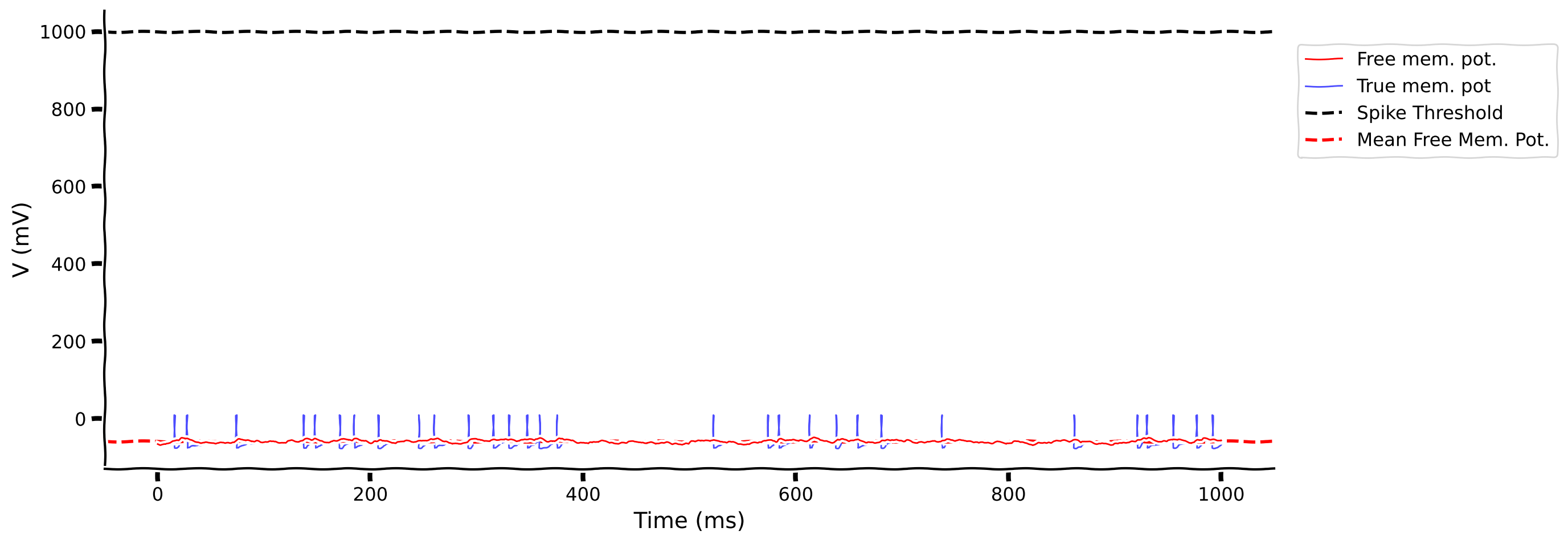
Coding Exercise 1.2: Measure the mean free membrane potential#

Let’s simulate the conductance-based LIF neuron with presynaptic spike trains generated by a Poisson_generator with rate 10 Hz for both excitatory and inhibitory inputs. Here, we choose 80 excitatory presynaptic spike trains and 20 inhibitory ones.

Previously, we’ve already learned that \(CV_{\rm ISI}\) can describe the irregularity of the output spike pattern. Now, we will introduce a new descriptor of the neuron membrane, i.e., the Free Membrane Potential (FMP) – the membrane potential of the neuron when its spike threshold is removed.

Although this is completely artificial, calculating this quantity allows us to get an idea of how strong the input is. We are mostly interested in knowing the mean and standard deviation (std.) of the FMP. In the exercise, you can visualize the FMP and membrane voltage with spike threshold.

# Get default parameters
pars = default_pars(T=1000.)

# Add parameters
pars['gE_bar'] = 2.4    # [nS]
pars['VE'] = 0.         # [mV] excitatory reversal potential
pars['tau_syn_E'] = 2.  # [ms]
pars['gI_bar'] = 2.4    # [nS]
pars['VI'] = -80.       # [mV] inhibitory reversal potential
pars['tau_syn_I'] = 5.  # [ms]

# Generate presynaptic spike trains
pre_spike_train_ex = Poisson_generator(pars, rate=10, n=80)
pre_spike_train_in = Poisson_generator(pars, rate=10, n=20)

# Simulate conductance-based LIF model
v, rec_spikes, gE, gI = run_LIF_cond(pars, 0, pre_spike_train_ex,
                                     pre_spike_train_in)

# Show spikes more clearly by setting voltage high
dt, range_t = pars['dt'], pars['range_t']
if rec_spikes.size:
  sp_num = (rec_spikes / dt).astype(int) - 1
  v[sp_num] = 10   # draw nicer spikes

####################################################################
## TODO for students: measure the free membrane potential
# In order to measure the free membrane potential, first,
# you should prevent the firing of the LIF neuron
# How to prevent a LIF neuron from firing? Increase the threshold pars['V_th'].
raise NotImplementedError("Student exercise: change threshold and calculate FMP")
####################################################################

# Change the threshold
pars['V_th'] = ...

# Calculate FMP
v_fmp, _, _, _ = run_LIF_cond(pars, ..., ..., ...)

my_illus_LIFSYN(pars, v_fmp, v)

Click for solution

Example output:

Submit your feedback#

Interactive Demo 1.2: Conductance-based LIF Explorer with different E/I input#

In the following, we can investigate how varying the ratio of excitatory to inhibitory inputs changes the firing rate and the spike time regularity (see the output text).

To change both the excitatory and inhibitory inputs, we will vary their firing rates. However, if you wish, you can vary the strength and/or the number of these connections as well.

Pay close attention to the mean free membrane potential (red dotted line) and its location with respect to the spike threshold (black dotted line).

Is there a relationship between the mean of the FMP and spike time irregularity (\(CV_{\rm ISI}\))? What happens when the mean of the FMP is above the spike threshold vs below?

Make sure you execute this cell to enable the widget!

Show code cell source Hide code cell source

# @markdown Make sure you execute this cell to enable the widget!

my_layout.width = '450px'
@widgets.interact(
    inh_rate=widgets.FloatSlider(20., min=10., max=60., step=5.,
                                 layout=my_layout),
    exc_rate=widgets.FloatSlider(10., min=2., max=20., step=2.,
                                 layout=my_layout)
)


def EI_isi_regularity(exc_rate, inh_rate):

  pars = default_pars(T=1000.)
  # Add parameters
  pars['gE_bar'] = 3.     # [nS]
  pars['VE'] = 0.         # [mV] excitatory reversal potential
  pars['tau_syn_E'] = 2.  # [ms]
  pars['gI_bar'] = 3.     # [nS]
  pars['VI'] = -80.       # [mV] inhibitory reversal potential
  pars['tau_syn_I'] = 5.  # [ms]

  pre_spike_train_ex = Poisson_generator(pars, rate=exc_rate, n=80)
  pre_spike_train_in = Poisson_generator(pars, rate=inh_rate, n=20)  # 4:1

  # Lets first simulate a neuron with identical input but with no spike
  # threshold by setting the threshold to a very high value
  # so that we can look at the free membrane potential
  pars['V_th'] = 1e3
  v_fmp, rec_spikes, gE, gI = run_LIF_cond(pars, 0, pre_spike_train_ex,
                                           pre_spike_train_in)

  # Now simulate a LIP with a regular spike threshold
  pars['V_th'] = -55.
  v, rec_spikes, gE, gI = run_LIF_cond(pars, 0, pre_spike_train_ex,
                                       pre_spike_train_in)
  dt, range_t = pars['dt'], pars['range_t']
  if rec_spikes.size:
      sp_num = (rec_spikes / dt).astype(int) - 1
      v[sp_num] = 10  # draw nicer spikes

  spike_rate = 1e3 * len(rec_spikes) / pars['T']

  cv_isi = 0.
  if len(rec_spikes) > 3:
    isi = np.diff(rec_spikes)
    cv_isi = np.std(isi) / np.mean(isi)

  print('\n')
  plt.figure(figsize=(15, 10))
  plt.subplot(211)
  plt.text(500, -35, f'Spike rate = {spike_rate:.3f} (sp/s), Mean of Free Mem Pot = {np.mean(v_fmp):.3f}',
           fontsize=16, fontweight='bold', horizontalalignment='center',
           verticalalignment='bottom')
  plt.text(500, -38.5, f'CV ISI = {cv_isi:.3f}, STD of Free Mem Pot = {np.std(v_fmp):.3f}',
           fontsize=16, fontweight='bold', horizontalalignment='center',
           verticalalignment='bottom')

  plt.plot(pars['range_t'], v_fmp, 'r', lw=1.,
           label='Free mem. pot.', zorder=2)
  plt.plot(pars['range_t'], v, 'b', lw=1.,
           label='mem. pot with spk thr', zorder=1, alpha=0.7)
  plt.axhline(pars['V_th'], 0, 1, color='k', lw=1., ls='--',
              label='Spike Threshold', zorder=1)
  plt.axhline(np.mean(v_fmp),0, 1, color='r', lw=1., ls='--',
              label='Mean Free Mem. Pot.', zorder=1)
  plt.ylim(-76, -39)
  plt.xlabel('Time (ms)')
  plt.ylabel('V (mV)')
  plt.legend(loc=[1.02, 0.68])

  plt.subplot(223)
  plt.plot(pars['range_t'][::3], gE[::3], 'r', lw=1)
  plt.xlabel('Time (ms)')
  plt.ylabel(r'$g_E$ (nS)')

  plt.subplot(224)
  plt.plot(pars['range_t'][::3], gI[::3], 'b', lw=1)
  plt.xlabel('Time (ms)')
  plt.ylabel(r'$g_I$ (nS)')

  plt.tight_layout()
  plt.show()

Click for solution

Submit your feedback#

Think! 1.2: Excitatory and Inhibitory Balance#

How much can you increase the spike pattern variability? Under what condition(s) might the neuron respond with Poisson-type spikes? Note that we injected Poisson-type spikes. (Think of the answer in terms of the ratio of the exc. and inh. input spike rates.)
Link to the balance of excitation and inhibition: one of the definitions of excitation and inhibition balance is that mean free membrane potential remains constant as excitatory and inhibitory input rates are increased. What do you think happens to the neuron firing rate as we change excitatory and inhibitory rates while keeping the neuron in balance? See Kuhn, Aertsen, and Rotter (2004) for much more on this.

Click for solution

Submit your feedback#

Section 2: Short-term synaptic plasticity#

Estimated timing to here from start of tutorial: 45 min

Above, we modeled synapses with fixed weights. Now we will explore synapses whose weights change in some input conditions.

Short-term plasticity (STP) is a phenomenon in which synaptic efficacy changes over time in a way that reflects the history of presynaptic activity. Two types of STP, with opposite effects on synaptic efficacy, have been experimentally observed. They are known as Short-Term Depression (STD) and Short-Term Facilitation (STF).

The mathematical model (for more information see here) of STP is based on the concept of a limited pool of synaptic resources available for transmission (\(R\)), such as, for example, the overall amount of synaptic vesicles at the presynaptic terminals. The amount of presynaptic resource changes in a dynamic fashion depending on the recent history of spikes.

Following a presynaptic spike, (i) the fraction \(u\) (release probability) of the available pool to be utilized increases due to spike-induced calcium influx to the presynaptic terminal, after which (ii) \(u\) is consumed to increase the post-synaptic conductance. Between spikes, \(u\) decays back to zero with time constant \(\tau_f\) and \(R\) recovers to 1 with time constant \(\tau_d\). In summary, the dynamics of excitatory (subscript \(E\)) STP are given by:

(297)#\[\begin{eqnarray} && \frac{du_E}{dt} &=& -\frac{u_E}{\tau_f} + U_0(1-u_E^-)\delta(t-t_{\rm sp}) \\[.5mm] && \frac{dR_E}{dt} &=& \frac{1-R_E}{\tau_d} - u_E^+ R_E^- \delta(t-t_{\rm sp}) \qquad (6) \\[.5mm] && \frac{dg_E(t)}{dt} &=& -\frac{g_E}{\tau_E} + \bar{g}_E u_E^+ R_E^- \delta(t-t_{\rm sp}) \end{eqnarray}\]

where \(U_0\) is a constant determining the increment of \(u\) produced by a spike. \(u_E^-\) and \(R_E^-\) denote the corresponding values just before the spike arrives, whereas \(u_E^+\) refers to the moment right after the spike. \(\bar{g}_E\) denotes the maximum excitatory conductance, and \(g_E(t)\) is calculated for all spiketimes \(k\), and decays over time with a time constant \(\tau_{E}\). Similarly, one can obtain the dynamics of inhibitory STP (i.e., by replacing the subscript \(E\) with \(I\)).

The interplay between the dynamics of \(u\) and \(R\) determines whether the joint effect of \(uR\) is dominated by depression or facilitation. In the parameter regime of \(\tau_d \gg \tau_f\) and for large \(U_0\), an initial spike incurs a large drop in \(R\) that takes a long time to recover; therefore, the synapse is STD-dominated. In the regime of \(\tau_d \ll \tau_f\) and for small \(U_0\), the synaptic efficacy is increased gradually by spikes, and consequently, the synapse is STF-dominated. This phenomenological model successfully reproduces the kinetic dynamics of depressed and facilitated synapses observed in many cortical areas.

We provide a helper function below, dynamic_syn that integrates the above equations using the Euler method (which you saw yesterday).

Execute this cell to get helper function dynamic_syn

Help on function dynamic_syn in module __main__:

dynamic_syn(g_bar, tau_syn, U0, tau_d, tau_f, pre_spike_train, dt)
    Short-term synaptic plasticity
    
    Args:
      g_bar           : synaptic conductance strength
      tau_syn         : synaptic time constant [ms]
      U0              : synaptic release probability at rest
      tau_d           : synaptic depression time constant of x [ms]
      tau_f           : synaptic facilitation time constantr of u [ms]
      pre_spike_train : total spike train (number) input
                        from presynaptic neuron
      dt              : time step [ms]
    
    Returns:
      u               : usage of releasable neurotransmitter
      R               : fraction of synaptic neurotransmitter resources available
      g               : postsynaptic conductance

Section 2.1: Short-term synaptic depression (STD)#

Interactive Demo 2.1: STD Explorer with input rate#

Below, an interactive demo that shows how Short-term synaptic depression (STD) changes for different firing rates of the presynaptic spike train and how the amplitude synaptic conductance \(g\) changes with every incoming spike until it reaches its stationary state.

How does the firing rate affect the synaptic efficacy? Does it matter if the neuron fires in a Poisson manner, rather than regularly?

Note: Poisson=True: for Poisson type and Poisson=False: for regular presynaptic spikes. You can check and uncheck the corresponding checkbox.

Make sure you execute this cell to enable the widget!

Click for solution

Submit your feedback#

Once, I asked an experimentalist about the experimental values of the PSP amplitude produced by a connection between two neocortical excitatory neurons. She asked: “At what frequency?” I was confused, but you will understand her question, now that you know that PSP amplitude depends on the spike history, and therefore on the spike rate of the presynaptic neuron.

Here, we will study how the ratio of the synaptic conductance corresponding to the first and 10th spikes change as a function of the presynaptic firing rate (experimentalists often take the ratio of first and second PSPs).

For computational efficiency, we assume that the presynaptic spikes are regular. This assumption means that we do not have to run multiple trials.

STD conductance ratio with different input rate

../../../_images/fc74286745f853ec884166a63734b8e7441ff079815498b39cd60c8ca6ef41ce.png

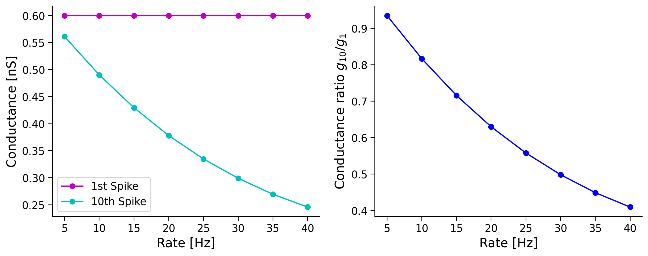
As we increase the input rate the ratio of the first to tenth spike is increased, because the tenth spike conductance becomes smaller. This is a clear evidence of synaptic depression, as using the same amount of current has a smaller effect on the neuron.

Section 2.2: Short-term synaptic facilitation (STF)#

Interactive Demo 2.2: STF explorer with input rate#

Below, we see an illustration of a short-term facilitation example. Take note of the change in the synaptic variables: U_0, tau_d, and tau_f.

for STD, U0=0.5, tau_d=100., tau_f=50.
for STP, U0=0.2, tau_d=100., tau_f=750.

How does the synaptic conductance change as we change the input rate? What do you observe in the case of a regular input and a Poisson type one?

Make sure you execute this cell to enable the widget!

Think! 2.2: Short-term synaptic facilitation vs. depression#

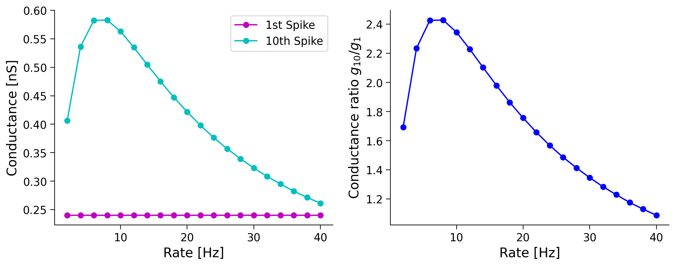
Here, we will study how the ratio of the synaptic conductance corresponding to the \(1^{st}\) and \(10^{th}\) spike changes as a function of the presynaptic rate.

Why does the ratio of the first and tenth spike conductance changes in a non-monotonic fashion for synapses with STF, even though it decreases monotonically for synapses with STD?

STF conductance ratio with different input rates

../../../_images/60440db1670173370087fddf21be0bbb1bb84f49d4e3699907d36bac09d8202b.png

Click for solution

Submit your feedback#

Summary#

Estimated timing of tutorial: 1 hour, 10 min

Congratulations! You have just finished the last tutorial of this day. Here, we saw how to model conductance-based synapses and also how to incorporate short-term dynamics in synaptic weights.

We covered the:

static synapses and how excitation and inhibition affect the neuronal output
mean- or fluctuation-driven regimes
short-term dynamics of synapses (both facilitation and depression)

Finally, we incorporated all the aforementioned tools to study how a change in presynaptic firing history affects the synaptic weights!

There are many interesting things that you can try on your own to develop a deeper understanding of biological synapses. A couple of those are mentioned below in the optional boxes – if you have time.

If you have time, you can look at a conductance-based LIF model with STP in the bonus sections below. There is also a whole bonus tutorial on spike timing dependent synaptic plasticity!

Bonus#

Bonus Section 1: Conductance-based LIF with STP#

Previously, we looked only at how the presynaptic firing rate affects the presynaptic resource availability and thereby the synaptic conductance. It is straightforward to imagine that, while the synaptic conductances are changing, the output of the postsynaptic neuron will change as well.

So, let’s put the STP on synapses impinging on an LIF neuron and see what happens.

Execute for helper function for conductance-based LIF neuron with STP-synapses

Show code cell source Hide code cell source

# @markdown Execute for helper function for conductance-based LIF neuron with STP-synapses

def run_LIF_cond_STP(pars, I_inj, pre_spike_train_ex, pre_spike_train_in):
  """
  conductance-based LIF dynamics

  Args:
    pars               : parameter dictionary
    I_inj              : injected current [pA]
                         The injected current here can be a value or an array
    pre_spike_train_ex : spike train input from presynaptic excitatory neuron (binary)
    pre_spike_train_in : spike train input from presynaptic inhibitory neuron (binary)

  Returns:
    rec_spikes : spike times
    rec_v      : mebrane potential
    gE         : postsynaptic excitatory conductance
    gI         : postsynaptic inhibitory conductance

  """

  # Retrieve parameters
  V_th, V_reset = pars['V_th'], pars['V_reset']
  tau_m, g_L = pars['tau_m'], pars['g_L']
  V_init, V_L = pars['V_init'], pars['E_L']
  gE_bar, gI_bar = pars['gE_bar'], pars['gI_bar']
  U0E, tau_dE, tau_fE = pars['U0_E'], pars['tau_d_E'], pars['tau_f_E']
  U0I, tau_dI, tau_fI = pars['U0_I'], pars['tau_d_I'], pars['tau_f_I']
  VE, VI = pars['VE'], pars['VI']
  tau_syn_E, tau_syn_I = pars['tau_syn_E'], pars['tau_syn_I']
  tref = pars['tref']

  dt, range_t = pars['dt'], pars['range_t']
  Lt = range_t.size

  nE = pre_spike_train_ex.shape[0]
  nI = pre_spike_train_in.shape[0]

  # compute conductance Excitatory synapses
  uE = np.zeros((nE, Lt))
  RE = np.zeros((nE, Lt))
  gE = np.zeros((nE, Lt))
  for ie in range(nE):
    u, R, g = dynamic_syn(gE_bar, tau_syn_E, U0E, tau_dE, tau_fE,
                          pre_spike_train_ex[ie, :], dt)

    uE[ie, :], RE[ie, :], gE[ie, :] = u, R, g

  gE_total = gE.sum(axis=0)

  # compute conductance Inhibitory synapses
  uI = np.zeros((nI, Lt))
  RI = np.zeros((nI, Lt))
  gI = np.zeros((nI, Lt))
  for ii in range(nI):
    u, R, g = dynamic_syn(gI_bar, tau_syn_I, U0I, tau_dI, tau_fI,
                          pre_spike_train_in[ii, :], dt)

    uI[ii, :], RI[ii, :], gI[ii, :] = u, R, g

  gI_total = gI.sum(axis=0)

  # Initialize
  v = np.zeros(Lt)
  v[0] = V_init
  Iinj = I_inj * np.ones(Lt)  # ensure I has length Lt

  # simulation
  rec_spikes = []  # recording spike times
  tr = 0.
  for it in range(Lt - 1):
    if tr > 0:
      v[it] = V_reset
      tr = tr - 1
    elif v[it] >= V_th:  # reset voltage and record spike event
      rec_spikes.append(it)
      v[it] = V_reset
      tr = tref / dt

    # calculate the increment of the membrane potential
    dv = (dt / tau_m) * (-(v[it] - V_L) \
                         - (gE_total[it + 1] / g_L) * (v[it] - VE) \
                         - (gI_total[it + 1] / g_L) * (v[it] - VI) + Iinj[it] / g_L)

    # update membrane potential
    v[it+1] = v[it] + dv

  rec_spikes = np.array(rec_spikes) * dt

  return v, rec_spikes, uE, RE, gE, RI, RI, gI


help(run_LIF_cond_STP)

Help on function run_LIF_cond_STP in module __main__:

run_LIF_cond_STP(pars, I_inj, pre_spike_train_ex, pre_spike_train_in)
    conductance-based LIF dynamics
    
    Args:
      pars               : parameter dictionary
      I_inj              : injected current [pA]
                           The injected current here can be a value or an array
      pre_spike_train_ex : spike train input from presynaptic excitatory neuron (binary)
      pre_spike_train_in : spike train input from presynaptic inhibitory neuron (binary)
    
    Returns:
      rec_spikes : spike times
      rec_v      : mebrane potential
      gE         : postsynaptic excitatory conductance
      gI         : postsynaptic inhibitory conductance

Bonus Interactive Demo: LIF with STP Explorer#

Here we have assumed that both excitatory and inhibitory synapses show short-term depression. Change the nature of synapses and study how spike pattern variability changes. In this demo, tau_d = 500*tau_ratio (ms) and tau_f = 300*tau_ratio (ms).

You should compare the output of this neuron with what you observed in the previous tutorial when synapses were assumed to be static.

Note: it will take slightly longer time to run each case

Make sure you execute this cell to enable the widget!

When we vary the tau_ratio we are increasing tau_f and tau_d i.e., by increasing tau_ratio we are increasing the synaptic depression. The effect is same on both Exc and Inh conductances. This is visible as a clear decrease in the firing rate of the neuron from 300-400ms onwards.

Not much happens in the beginning because synaptic depression takes some time to become visible.

It is curious that while both excitatory and inhibitory conductances have depressed but output firing rate has still decreased.

There are two explanations of this:

Excitation has depressed more than inhibition from their starting values.
Because synaptic conductances have depressed, membrane fluctuation size has decreased.

Which is the more likely reason?

Submit your feedback#

Will the neuron show higher irregularity if the synapses have STP?

Try calculating the \(CV_{\rm ISI}\) for different tau_ratio after simulating the LIF neuron with STP (Hint:run_LIF_cond_STP will help you understand the irregularity).

Functional implications of short-term dynamics of synapses

As you have seen above, if the firing rate is stationary, the synaptic conductance quickly reaches a fixed point. On the other hand, if the firing rate transiently changes, synaptic conductance will vary – even if the change is as short as a single inter-spike-interval. Such small changes can be observed in a single neuron when input spikes are regular and periodic. If the input spikes are Poissonian, then one may have to perform an average over several neurons.

Come up with other functions that short-term dynamics of synapses can be used to implement and implement them.

Tutorial 3: Synaptic transmission - Models of static and dynamic synapses

Contents

Tutorial 3: Synaptic transmission - Models of static and dynamic synapses#

Tutorial Objectives#

Setup#

Install and import feedback gadget#

Figure Settings#

Plotting Functions#

Helper Functions#

Section 0: Static and Dynamic Synapses#

Video 1: Static and dynamic synapses#

Submit your feedback#

Section 1: Static synapses#

Section 1.1: Simulate synaptic conductance dynamics#

Section 1.2: Simulate LIF neuron with conductance-based synapses#

Coding Exercise 1.2: Measure the mean free membrane potential#

Submit your feedback#

Interactive Demo 1.2: Conductance-based LIF Explorer with different E/I input#

Submit your feedback#

Think! 1.2: Excitatory and Inhibitory Balance#

Submit your feedback#

Section 2: Short-term synaptic plasticity#

Section 2.1: Short-term synaptic depression (STD)#

Interactive Demo 2.1: STD Explorer with input rate#

Submit your feedback#

Section 2.2: Short-term synaptic facilitation (STF)#

Interactive Demo 2.2: STF explorer with input rate#

Think! 2.2: Short-term synaptic facilitation vs. depression#

Submit your feedback#

Summary#

Bonus#

Bonus Section 1: Conductance-based LIF with STP#

Bonus Interactive Demo: LIF with STP Explorer#

Submit your feedback#