Tutorial 2: Wilson-Cowan Model

Tutorial 2: Wilson-Cowan Model#

Week 2, Day 4: Dynamic Networks

By Neuromatch Academy

Content creators: Qinglong Gu, Songtin Li, Arvind Kumar, John Murray, Julijana Gjorgjieva

Content reviewers: Maryam Vaziri-Pashkam, Ella Batty, Lorenzo Fontolan, Richard Gao, Spiros Chavlis, Michael Waskom, Siddharth Suresh

Production editors: Gagana B, Spiros Chavlis

Tutorial Objectives#

Estimated timing of tutorial: 1 hour, 35 minutes

In the previous tutorial, you became familiar with a neuronal network consisting of only an excitatory population. Here, we extend the approach we used to include both excitatory and inhibitory neuronal populations in our network. A simple, yet powerful model to study the dynamics of two interacting populations of excitatory and inhibitory neurons, is the so-called Wilson-Cowan rate model, which will be the subject of this tutorial.

The objectives of this tutorial are to:

Write the Wilson-Cowan equations for the firing rate dynamics of a 2D system composed of an excitatory (E) and an inhibitory (I) population of neurons
Simulate the dynamics of the system, i.e., Wilson-Cowan model.
Plot the frequency-current (F-I) curves for both populations (i.e., E and I).
Visualize and inspect the behavior of the system using phase plane analysis, vector fields, and nullclines.

Bonus steps:

Find and plot the fixed points of the Wilson-Cowan model.
Investigate the stability of the Wilson-Cowan model by linearizing its dynamics and examining the Jacobian matrix.
Learn how the Wilson-Cowan model can reach an oscillatory state.

Bonus steps (applications):

Visualize the behavior of an Inhibition-stabilized network.
Simulate working memory using the Wilson-Cowan model.

Reference paper:

Wilson, H., and Cowan, J. (1972). Excitatory and inhibitory interactions in localized populations of model neurons. Biophysical Journal 12. doi: 10.1016/S0006-3495(72)86068-5.

Setup#

Install and import feedback gadget#

# Imports
import matplotlib.pyplot as plt
import numpy as np
import scipy.optimize as opt  # root-finding algorithm

Figure Settings#

Plotting Functions#

Show code cell source Hide code cell source

# @title Plotting Functions

def plot_FI_inverse(x, a, theta):
  f, ax = plt.subplots()
  ax.plot(x, F_inv(x, a=a, theta=theta))
  ax.set(xlabel="$x$", ylabel="$F^{-1}(x)$")


def plot_FI_EI(x, FI_exc, FI_inh):
  plt.figure()
  plt.plot(x, FI_exc, 'b', label='E population')
  plt.plot(x, FI_inh, 'r', label='I population')
  plt.legend(loc='lower right')
  plt.xlabel('x (a.u.)')
  plt.ylabel('F(x)')
  plt.show()


def my_test_plot(t, rE1, rI1, rE2, rI2):

  plt.figure()
  ax1 = plt.subplot(211)
  ax1.plot(pars['range_t'], rE1, 'b', label='E population')
  ax1.plot(pars['range_t'], rI1, 'r', label='I population')
  ax1.set_ylabel('Activity')
  ax1.legend(loc='best')

  ax2 = plt.subplot(212, sharex=ax1, sharey=ax1)
  ax2.plot(pars['range_t'], rE2, 'b', label='E population')
  ax2.plot(pars['range_t'], rI2, 'r', label='I population')
  ax2.set_xlabel('t (ms)')
  ax2.set_ylabel('Activity')
  ax2.legend(loc='best')

  plt.tight_layout()
  plt.show()


def plot_nullclines(Exc_null_rE, Exc_null_rI, Inh_null_rE, Inh_null_rI):

  plt.figure()
  plt.plot(Exc_null_rE, Exc_null_rI, 'b', label='E nullcline')
  plt.plot(Inh_null_rE, Inh_null_rI, 'r', label='I nullcline')
  plt.xlabel(r'$r_E$')
  plt.ylabel(r'$r_I$')
  plt.legend(loc='best')
  plt.show()


def my_plot_nullcline(pars):
  Exc_null_rE = np.linspace(-0.01, 0.96, 100)
  Exc_null_rI = get_E_nullcline(Exc_null_rE, **pars)
  Inh_null_rI = np.linspace(-.01, 0.8, 100)
  Inh_null_rE = get_I_nullcline(Inh_null_rI, **pars)

  plt.plot(Exc_null_rE, Exc_null_rI, 'b', label='E nullcline')
  plt.plot(Inh_null_rE, Inh_null_rI, 'r', label='I nullcline')
  plt.xlabel(r'$r_E$')
  plt.ylabel(r'$r_I$')
  plt.legend(loc='best')


def my_plot_vector(pars, my_n_skip=2, myscale=5):
  EI_grid = np.linspace(0., 1., 20)
  rE, rI = np.meshgrid(EI_grid, EI_grid)
  drEdt, drIdt = EIderivs(rE, rI, **pars)

  n_skip = my_n_skip

  plt.quiver(rE[::n_skip, ::n_skip], rI[::n_skip, ::n_skip],
             drEdt[::n_skip, ::n_skip], drIdt[::n_skip, ::n_skip],
             angles='xy', scale_units='xy', scale=myscale, facecolor='c')

  plt.xlabel(r'$r_E$')
  plt.ylabel(r'$r_I$')


def my_plot_trajectory(pars, mycolor, x_init, mylabel):
  pars = pars.copy()
  pars['rE_init'], pars['rI_init'] = x_init[0], x_init[1]
  rE_tj, rI_tj = simulate_wc(**pars)

  plt.plot(rE_tj, rI_tj, color=mycolor, label=mylabel)
  plt.plot(x_init[0], x_init[1], 'o', color=mycolor, ms=8)
  plt.xlabel(r'$r_E$')
  plt.ylabel(r'$r_I$')


def my_plot_trajectories(pars, dx, n, mylabel):
  """
  Solve for I along the E_grid from dE/dt = 0.

  Expects:
  pars    : Parameter dictionary
  dx      : increment of initial values
  n       : n*n trjectories
  mylabel : label for legend

  Returns:
    figure of trajectory
  """
  pars = pars.copy()
  for ie in range(n):
    for ii in range(n):
      pars['rE_init'], pars['rI_init'] = dx * ie, dx * ii
      rE_tj, rI_tj = simulate_wc(**pars)
      if (ie == n-1) & (ii == n-1):
          plt.plot(rE_tj, rI_tj, 'gray', alpha=0.8, label=mylabel)
      else:
          plt.plot(rE_tj, rI_tj, 'gray', alpha=0.8)

  plt.xlabel(r'$r_E$')
  plt.ylabel(r'$r_I$')


def plot_complete_analysis(pars):
  plt.figure(figsize=(7.7, 6.))

  # plot example trajectories
  my_plot_trajectories(pars, 0.2, 6,
                       'Sample trajectories \nfor different init. conditions')
  my_plot_trajectory(pars, 'orange', [0.6, 0.8],
                     'Sample trajectory for \nlow activity')
  my_plot_trajectory(pars, 'm', [0.6, 0.6],
                     'Sample trajectory for \nhigh activity')

  # plot nullclines
  my_plot_nullcline(pars)

  # plot vector field
  EI_grid = np.linspace(0., 1., 20)
  rE, rI = np.meshgrid(EI_grid, EI_grid)
  drEdt, drIdt = EIderivs(rE, rI, **pars)
  n_skip = 2
  plt.quiver(rE[::n_skip, ::n_skip], rI[::n_skip, ::n_skip],
             drEdt[::n_skip, ::n_skip], drIdt[::n_skip, ::n_skip],
             angles='xy', scale_units='xy', scale=5., facecolor='c')

  plt.legend(loc=[1.02, 0.57], handlelength=1)
  plt.show()


def plot_fp(x_fp, position=(0.02, 0.1), rotation=0):
  plt.plot(x_fp[0], x_fp[1], 'ko', ms=8)
  plt.text(x_fp[0] + position[0], x_fp[1] + position[1],
           f'Fixed Point1=\n({x_fp[0]:.3f}, {x_fp[1]:.3f})',
           horizontalalignment='center', verticalalignment='bottom',
           rotation=rotation)

Helper Functions#

The helper functions included:

Parameter dictionary: default_pars(**kwargs). You can use:
- pars = default_pars() to get all the parameters, and then you can execute print(pars) to check these parameters.
- pars = default_pars(T=T_sim, dt=time_step) to set a different simulation time and time step
- After pars = default_pars(), use par['New_para'] = value to add a new parameter with its value
- Pass to functions that accept individual parameters with func(**pars)
F-I curve: F(x, a, theta)
Derivative of the F-I curve: dF(x, a, theta)

Section 1: Wilson-Cowan model of excitatory and inhibitory populations#

Video 1: Phase analysis of the Wilson-Cowan E-I model#

Submit your feedback#

This video explains how to model a network with interacting populations of excitatory and inhibitory neurons (the Wilson-Cowan model). It shows how to solve the network activity vs. time and introduces the phase plane in two dimensions.

Section 1.1: Mathematical description of the WC model#

Estimated timing to here from start of tutorial: 12 min

Click here for text recap of relevant part of video

Many of the rich dynamics recorded in the brain are generated by the interaction of excitatory and inhibitory subtype neurons. Here, similar to what we did in the previous tutorial, we will model two coupled populations of E and I neurons (Wilson-Cowan model). We can write two coupled differential equations, each representing the dynamics of the excitatory or inhibitory population:

(323)#\[\begin{align} \tau_E \frac{dr_E}{dt} &= -r_E + F_E(w_{EE}r_E -w_{EI}r_I + I^{\text{ext}}_E;a_E,\theta_E)\\ \tau_I \frac{dr_I}{dt} &= -r_I + F_I(w_{IE}r_E -w_{II}r_I + I^{\text{ext}}_I;a_I,\theta_I) \qquad (1) \end{align}\]

\(r_E(t)\) represents the average activation (or firing rate) of the excitatory population at time \(t\), and \(r_I(t)\) the activation (or firing rate) of the inhibitory population. The parameters \(\tau_E\) and \(\tau_I\) control the timescales of the dynamics of each population. Connection strengths are given by: \(w_{EE}\) (E \(\rightarrow\) E), \(w_{EI}\) (I \(\rightarrow\) E), \(w_{IE}\) (E \(\rightarrow\) I), and \(w_{II}\) (I \(\rightarrow\) I). The terms \(w_{EI}\) and \(w_{IE}\) represent connections from inhibitory to excitatory population and vice versa, respectively. The transfer functions (or F-I curves) \(F_E(x;a_E,\theta_E)\) and \(F_I(x;a_I,\theta_I)\) can be different for the excitatory and the inhibitory populations.

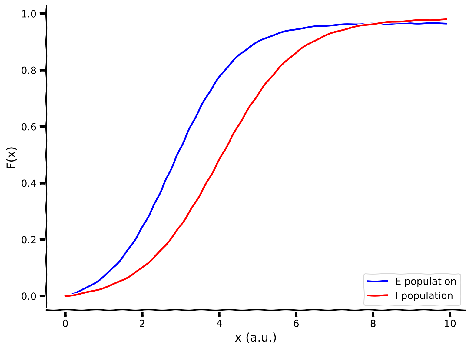
Coding Exercise 1.1: Plot out the F-I curves for the E and I populations#

Let’s first plot out the F-I curves for the E and I populations using the helper function F with default parameter values.

help(F)

Help on function F in module __main__:

F(x, a, theta)
    Population activation function, F-I curve
    
    Args:
      x     : the population input
      a     : the gain of the function
      theta : the threshold of the function
    
    Returns:
      f     : the population activation response f(x) for input x

pars = default_pars()
x = np.arange(0, 10, .1)

print(pars['a_E'], pars['theta_E'])
print(pars['a_I'], pars['theta_I'])

###################################################################
# TODO for students: compute and plot the F-I curve here          #
# Note: aE, thetaE, aI and theta_I are in the dictionary 'pairs'   #
raise NotImplementedError('student exercise: compute F-I curves of excitatory and inhibitory populations')
###################################################################

# Compute the F-I curve of the excitatory population
FI_exc = ...

# Compute the F-I curve of the inhibitory population
FI_inh = ...

# Visualize
plot_FI_EI(x, FI_exc, FI_inh)

Click for solution

Example output:

Submit your feedback#

Section 1.2: Simulation scheme for the Wilson-Cowan model#

Estimated timing to here from start of tutorial: 20 min

Once again, we can integrate our equations numerically. Using the Euler method, the dynamics of E and I populations can be simulated on a time-grid of stepsize \(\Delta t\). The updates for the activity of the excitatory and the inhibitory populations can be written as:

(324)#\[\begin{align} r_E[k+1] &= r_E[k] + \Delta r_E[k]\\ r_I[k+1] &= r_I[k] + \Delta r_I[k] \end{align}\]

with the increments

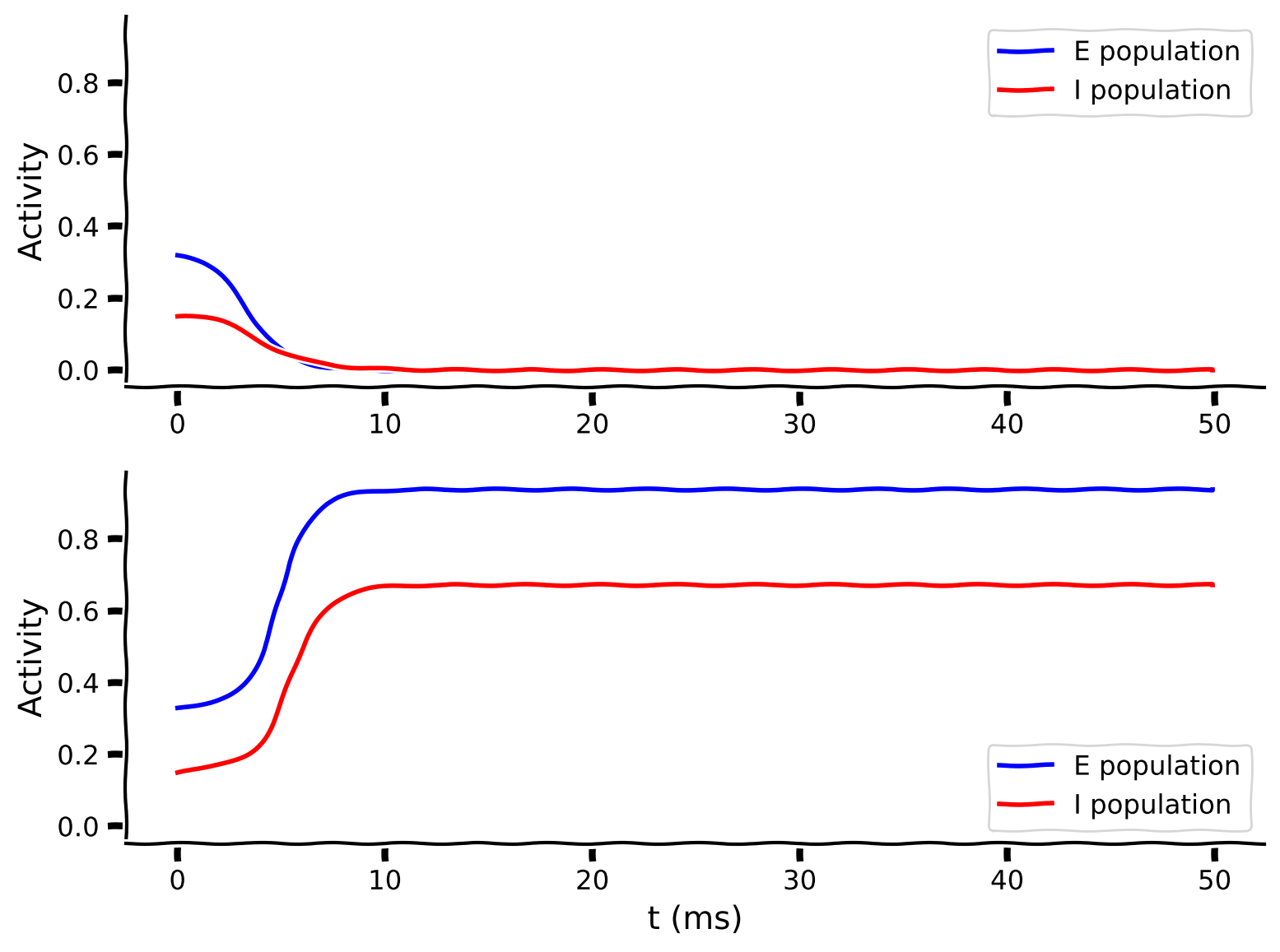
(325)#\[\begin{align} \Delta r_E[k] &= \frac{\Delta t}{\tau_E}[-r_E[k] + F_E(w_{EE}r_E[k] -w_{EI}r_I[k] + I^{\text{ext}}_E[k];a_E,\theta_E)]\\ \Delta r_I[k] &= \frac{\Delta t}{\tau_I}[-r_I[k] + F_I(w_{IE}r_E[k] -w_{II}r_I[k] + I^{\text{ext}}_I[k];a_I,\theta_I)] \end{align}\]

Coding Exercise 1.2: Numerically integrate the Wilson-Cowan equations#

We will implement this numerical simulation of our equations and visualize two simulations with similar initial points.

def simulate_wc(tau_E, a_E, theta_E, tau_I, a_I, theta_I,
                wEE, wEI, wIE, wII, I_ext_E, I_ext_I,
                rE_init, rI_init, dt, range_t, **other_pars):
  """
  Simulate the Wilson-Cowan equations

  Args:
    Parameters of the Wilson-Cowan model

  Returns:
    rE, rI (arrays) : Activity of excitatory and inhibitory populations
  """
  # Initialize activity arrays
  Lt = range_t.size
  rE = np.append(rE_init, np.zeros(Lt - 1))
  rI = np.append(rI_init, np.zeros(Lt - 1))
  I_ext_E = I_ext_E * np.ones(Lt)
  I_ext_I = I_ext_I * np.ones(Lt)

  # Simulate the Wilson-Cowan equations
  for k in range(Lt - 1):

    ########################################################################
    # TODO for students: compute drE and drI and remove the error
    raise NotImplementedError("Student exercise: compute the change in E/I")
    ########################################################################

    # Calculate the derivative of the E population
    drE = ...

    # Calculate the derivative of the I population
    drI = ...

    # Update using Euler's method
    rE[k + 1] = rE[k] + drE
    rI[k + 1] = rI[k] + drI

  return rE, rI


pars = default_pars()

# Simulate first trajectory
rE1, rI1 = simulate_wc(**default_pars(rE_init=.32, rI_init=.15))

# Simulate second trajectory
rE2, rI2 = simulate_wc(**default_pars(rE_init=.33, rI_init=.15))

# Visualize
my_test_plot(pars['range_t'], rE1, rI1, rE2, rI2)

Click for solution

Example output:

Submit your feedback#

The two plots above show the temporal evolution of excitatory (\(r_E\), blue) and inhibitory (\(r_I\), red) activity for two different sets of initial conditions.

Interactive Demo 1.2: population trajectories with different initial values#

In this interactive demo, we will simulate the Wilson-Cowan model and plot the trajectories of each population. We change the initial activity of the excitatory population.

What happens to the E and I population trajectories with different initial conditions?

Make sure you execute this cell to enable the widget!

Click for solution

Submit your feedback#

Think! 1.2#

It is evident that the steady states of the neuronal response can be different when different initial states are chosen. Why is that?

We will discuss this in the next section but try to think about it first.

Section 2: Phase plane analysis#

Estimated timing to here from start of tutorial: 45 min

Just like we used a graphical method to study the dynamics of a 1-D system in the previous tutorial, here we will learn a graphical approach called phase plane analysis to study the dynamics of a 2-D system like the Wilson-Cowan model. You have seen this before in the pre-reqs calculus day and on the Linear Systems day

So far, we have plotted the activities of the two populations as a function of time, i.e., in the Activity-t plane, either the \((t, r_E(t))\) plane or the \((t, r_I(t))\) one. Instead, we can plot the two activities \(r_E(t)\) and \(r_I(t)\) against each other at any time point \(t\). This characterization in the rI-rE plane \((r_I(t), r_E(t))\) is called the phase plane. Each line in the phase plane indicates how both \(r_E\) and \(r_I\) evolve with time.

Video 2: Nullclines and Vector Fields#

Submit your feedback#

Interactive Demo 2: From the Activity - time plane to the \(r_I\) - \(r_E\) phase plane#

In this demo, we will visualize the system dynamics using both the Activity-time and the (rE, rI) phase plane. The circles indicate the activities at a given time \(t\), while the lines represent the evolution of the system for the entire duration of the simulation.

Move the time slider to better understand how the top plot relates to the bottom plot. Does the bottom plot have explicit information about time? What information does it give us?

Make sure you execute this cell to enable the widget!

Click for solution

Submit your feedback#

Section 2.1: Nullclines of the Wilson-Cowan Equations#

Estimated timing to here from start of tutorial: 1 hour, 3 min

An important concept in the phase plane analysis is the “nullcline” which is defined as the set of points in the phase plane where the activity of one population (but not necessarily the other) does not change.

In other words, the \(E\) and \(I\) nullclines of Equation \((1)\) are defined as the points where \(\displaystyle{\frac{dr_E}{dt}}=0\), for the excitatory nullcline, or \(\displaystyle\frac{dr_I}{dt}=0\) for the inhibitory nullcline. That is:

(326)#\[\begin{align} -r_E + F_E(w_{EE}r_E -w_{EI}r_I + I^{\text{ext}}_E;a_E,\theta_E) &= 0 \qquad (2)\\[1mm] -r_I + F_I(w_{IE}r_E -w_{II}r_I + I^{\text{ext}}_I;a_I,\theta_I) &= 0 \qquad (3) \end{align}\]

Coding Exercise 2.1: Compute the nullclines of the Wilson-Cowan model#

In the next exercise, we will compute and plot the nullclines of the E and I population.

Along the nullcline of excitatory population Equation \(2\), you can calculate the inhibitory activity by rewriting Equation \(2\) into

(327)#\[\begin{align} r_I = \frac{1}{w_{EI}}\big{[}w_{EE}r_E - F_E^{-1}(r_E; a_E,\theta_E) + I^{\text{ext}}_E \big{]}. \qquad(4) \end{align}\]

where \(F_E^{-1}(r_E; a_E,\theta_E)\) is the inverse of the excitatory transfer function (defined below). Equation \(4\) defines the \(r_E\) nullcline.

Along the nullcline of inhibitory population Equation \(3\), you can calculate the excitatory activity by rewriting Equation \(3\) into

(328)#\[\begin{align} r_E = \frac{1}{w_{IE}} \big{[} w_{II}r_I + F_I^{-1}(r_I;a_I,\theta_I) - I^{\text{ext}}_I \big{]} \qquad (5) \end{align}\]

shere \(F_I^{-1}(r_I; a_I,\theta_I)\) is the inverse of the inhibitory transfer function (defined below). Equation \(5\) defines the \(I\) nullcline.

Note that, when computing the nullclines with Equations 4-5, we also need to calculate the inverse of the transfer functions.

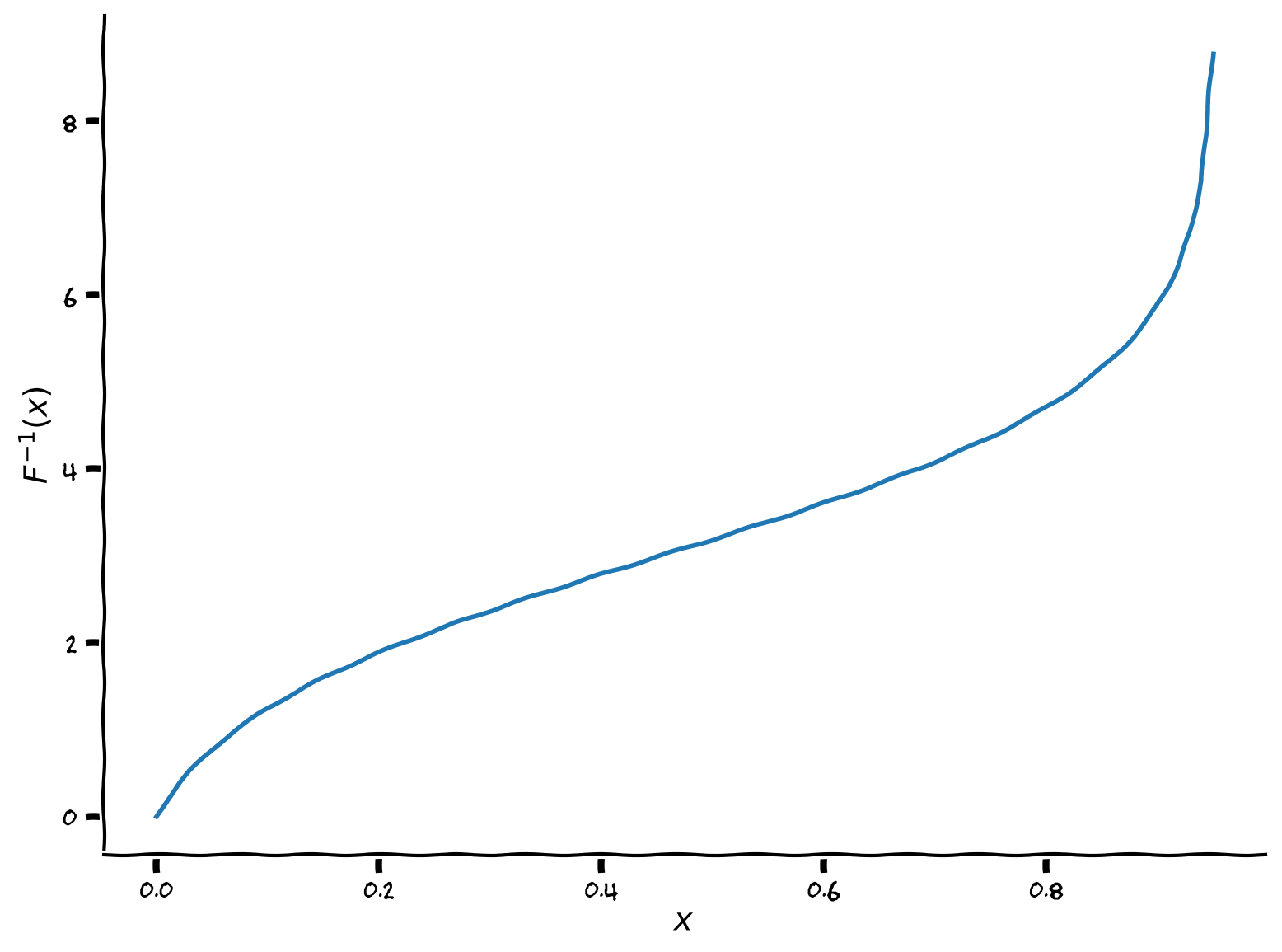
The inverse of the sigmoid shaped f-I function that we have been using is:

(329)#\[\begin{equation} F^{-1}(x; a, \theta) = -\frac{1}{a} \ln \left[ \frac{1}{x + \displaystyle \frac{1}{1+\text{e}^{a\theta}}} - 1 \right] + \theta \qquad (6) \end{equation}\]

The first step is to implement the inverse transfer function:

def F_inv(x, a, theta):
  """
  Args:
    x         : the population input
    a         : the gain of the function
    theta     : the threshold of the function

  Returns:
    F_inverse : value of the inverse function
  """

  #########################################################################
  # TODO for students: compute F_inverse
  raise NotImplementedError("Student exercise: compute the inverse of F(x)")
  #########################################################################

  # Calculate Finverse (ln(x) can be calculated as np.log(x))
  F_inverse = ...

  return F_inverse


# Set parameters
pars = default_pars()
x = np.linspace(1e-6, 1, 100)

# Get inverse and visualize
plot_FI_inverse(x, a=1, theta=3)

Click for solution

Now you can compute the nullclines, using Equations 4-5 (repeated here for ease of access):

(330)#\[\begin{align} r_I &= \frac{1}{w_{EI}}\big{[}w_{EE}r_E - F_E^{-1}(r_E; a_E,\theta_E) + I^{\text{ext}}_E \big{]} &\qquad(4) \\ r_E &= \frac{1}{w_{IE}} \big{[} w_{II}r_I + F_I^{-1}(r_I;a_I,\theta_I) - I^{\text{ext}}_I \big{]} &\qquad (5) \end{align}\]

def get_E_nullcline(rE, a_E, theta_E, wEE, wEI, I_ext_E, **other_pars):
  """
  Solve for rI along the rE from drE/dt = 0.

  Args:
    rE    : response of excitatory population
    a_E, theta_E, wEE, wEI, I_ext_E : Wilson-Cowan excitatory parameters
    Other parameters are ignored

  Returns:
    rI    : values of inhibitory population along the nullcline on the rE
  """
  #########################################################################
  # TODO for students: compute rI for rE nullcline and disable the error
  raise NotImplementedError("Student exercise: compute the E nullcline")
  #########################################################################

  # calculate rI for E nullclines on rI
  rI = ...

  return rI


def get_I_nullcline(rI, a_I, theta_I, wIE, wII, I_ext_I, **other_pars):
  """
  Solve for E along the rI from dI/dt = 0.

  Args:
    rI    : response of inhibitory population
    a_I, theta_I, wIE, wII, I_ext_I : Wilson-Cowan inhibitory parameters
    Other parameters are ignored

  Returns:
    rE    : values of the excitatory population along the nullcline on the rI
  """
  #########################################################################
  # TODO for students: compute rI for rE nullcline and disable the error
  raise NotImplementedError("Student exercise: compute the I nullcline")
  #########################################################################

  # calculate rE for I nullclines on rI
  rE = ...

  return rE


# Set parameters
pars = default_pars()
Exc_null_rE = np.linspace(-0.01, 0.96, 100)
Inh_null_rI = np.linspace(-.01, 0.8, 100)

# Compute nullclines
Exc_null_rI = get_E_nullcline(Exc_null_rE, **pars)
Inh_null_rE = get_I_nullcline(Inh_null_rI, **pars)

# Visualize
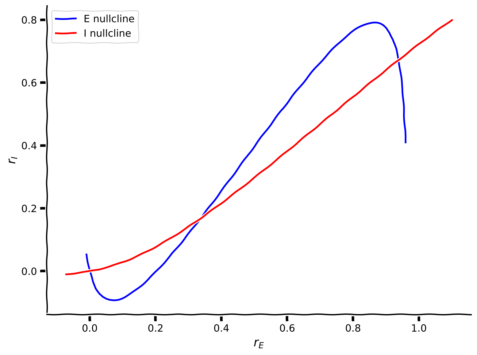
plot_nullclines(Exc_null_rE, Exc_null_rI, Inh_null_rE, Inh_null_rI)

Click for solution

Example output:

Submit your feedback#

Note that by definition along the blue line in the phase-plane spanned by \(r_E, r_I\), \(\displaystyle{\frac{dr_E(t)}{dt}} = 0\), therefore, it is called a nullcline.

That is, the blue nullcline divides the phase-plane spanned by \(r_E, r_I\) into two regions: on one side of the nullcline \(\displaystyle{\frac{dr_E(t)}{dt}} > 0\) and on the other side \(\displaystyle{\frac{dr_E(t)}{dt}} < 0\).

The same is true for the red line along which \(\displaystyle{\frac{dr_I(t)}{dt}} = 0\). That is, the red nullcline divides the phase-plane spanned by \(r_E, r_I\) into two regions: on one side of the nullcline \(\displaystyle{\frac{dr_I(t)}{dt}} > 0\) and on the other side \(\displaystyle{\frac{dr_I(t)}{dt}} < 0\).

Section 2.2: Vector field#

Estimated timing to here from start of tutorial: 1 hour, 20 min

How can the phase plane and the nullcline curves help us understand the behavior of the Wilson-Cowan model?

Click here for text recap of relevant part of video

The activities of the \(E\) and \(I\) populations \(r_E(t)\) and \(r_I(t)\) at each time point \(t\) correspond to a single point in the phase plane, with coordinates \((r_E(t),r_I(t))\). Therefore, the time-dependent trajectory of the system can be described as a continuous curve in the phase plane, and the tangent vector to the trajectory, which is defined as the vector \(\bigg{(}\displaystyle{\frac{dr_E(t)}{dt},\frac{dr_I(t)}{dt}}\bigg{)}\), indicates the direction towards which the activity is evolving and how fast is the activity changing along each axis. In fact, for each point \((E,I)\) in the phase plane, we can compute the tangent vector \(\bigg{(}\displaystyle{\frac{dr_E}{dt},\frac{dr_I}{dt}}\bigg{)}\), which indicates the behavior of the system when it traverses that point.

The map of tangent vectors in the phase plane is called vector field. The behavior of any trajectory in the phase plane is determined by i) the initial conditions \((r_E(0),r_I(0))\), and ii) the vector field \(\bigg{(}\displaystyle{\frac{dr_E(t)}{dt},\frac{dr_I(t)}{dt}}\bigg{)}\).

In general, the value of the vector field at a particular point in the phase plane is represented by an arrow. The orientation and the size of the arrow reflect the direction and the norm of the vector, respectively.

Coding Exercise 2.2: Compute and plot the vector field \(\displaystyle{\Big{(}\frac{dr_E}{dt}, \frac{dr_I}{dt} \Big{)}}\)#

Note that

(331)#\[\begin{align} \frac{dr_E}{dt} &= [-r_E + F_E(w_{EE}r_E -w_{EI}r_I + I^{\text{ext}}_E;a_E,\theta_E)]\frac{1}{\tau_E}\\ \frac{dr_I}{dt} &= [-r_I + F_I(w_{IE}r_E -w_{II}r_I + I^{\text{ext}}_I;a_I,\theta_I)]\frac{1}{\tau_I} \end{align}\]

def EIderivs(rE, rI,
             tau_E, a_E, theta_E, wEE, wEI, I_ext_E,
             tau_I, a_I, theta_I, wIE, wII, I_ext_I,
             **other_pars):
  """Time derivatives for E/I variables (dE/dt, dI/dt)."""
  ######################################################################
  # TODO for students: compute drEdt and drIdt and disable the error
  raise NotImplementedError("Student exercise: compute the vector field")
  ######################################################################

  # Compute the derivative of rE
  drEdt = ...

  # Compute the derivative of rI
  drIdt = ...

  return drEdt, drIdt


# Create vector field using EIderivs
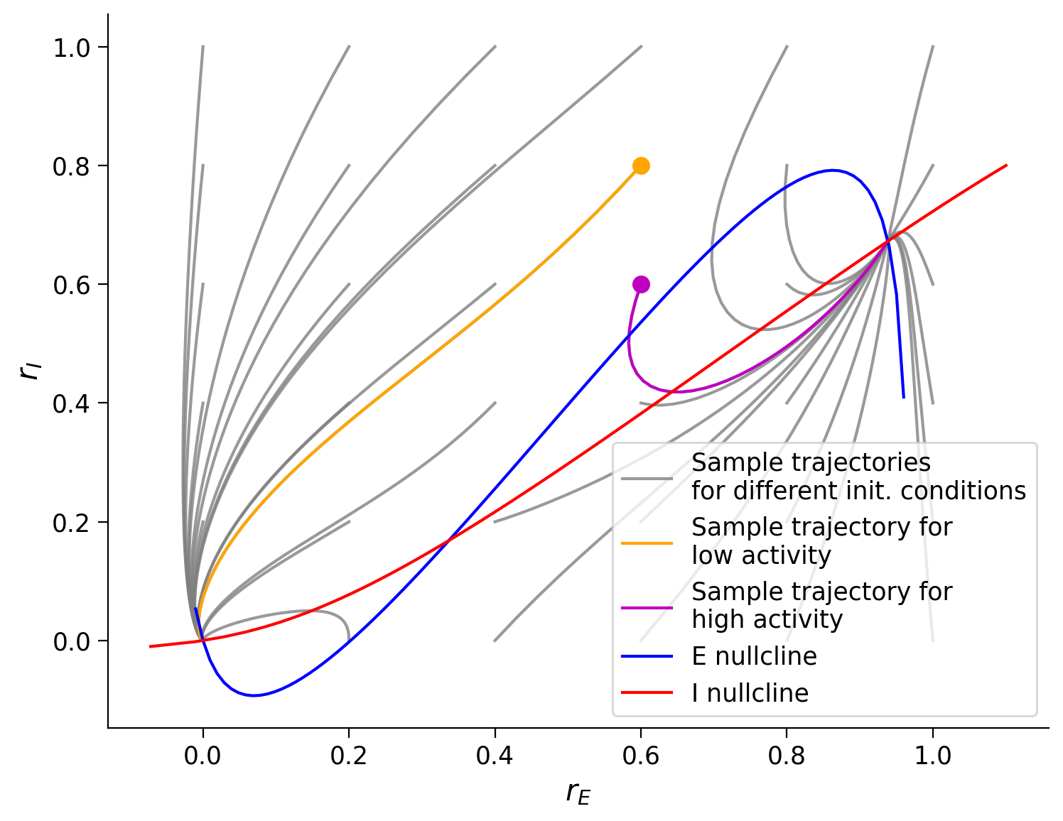
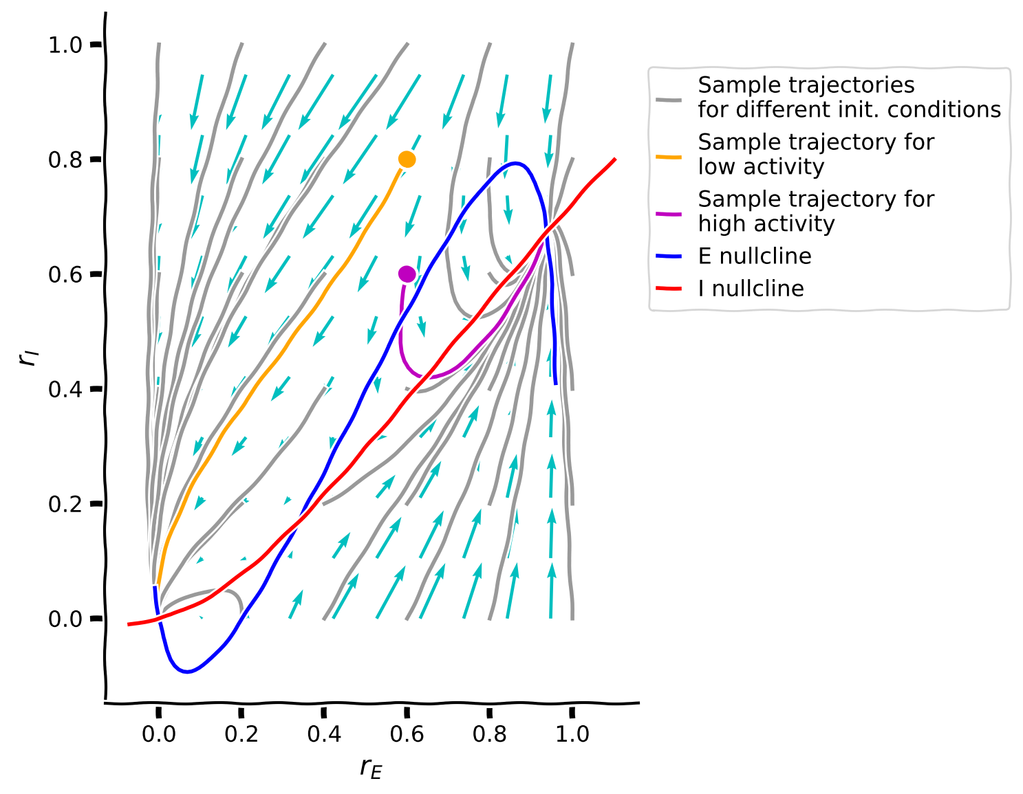
plot_complete_analysis(default_pars())

Click for solution

Example output:

Submit your feedback#

The last phase plane plot shows us that:

Trajectories seem to follow the direction of the vector field.
Different trajectories eventually always reach one of two points depending on the initial conditions.
The two points where the trajectories converge are the intersection of the two nullcline curves.

Think! 2.2: Analyzing the vector field#

There are, in total, three intersection points, meaning that the system has three fixed points.

One of the fixed points (the one in the middle) is never the final state of a trajectory. Why is that?
Why do the arrows tend to get smaller as they approach the fixed points?

Click for solution

Submit your feedback#

Summary#

Estimated timing of tutorial: 1 hour, 35 minutes

Congratulations! You have finished the fourth day of the second week of the neuromatch academy! Here, you learned how to simulate a rate based model consisting of excitatory and inhibitory population of neurons.

In the last tutorial on dynamical neuronal networks you learned to:

Implement and simulate a 2D system composed of an E and an I population of neurons using the Wilson-Cowan model
Plot the frequency-current (F-I) curves for both populations
Examine the behavior of the system using phase plane analysis, vector fields, and nullclines.

Do you have more time? Have you finished early? We have more fun material for you!

In the bonus tutorial, there are some, more advanced concepts on dynamical systems:

You will learn how to find the fixed points on such a system, and to investigate its stability by linearizing its dynamics and examining the Jacobian matrix.
You will identify conditions under which the Wilson-Cowan model can exhibit oscillations.

If you need even more, there are two applications of the Wilson-Cowan model:

Visualization of an Inhibition-stabilized network
Simulation of working memory

Tutorial 2: Wilson-Cowan Model

Contents

Tutorial 2: Wilson-Cowan Model#

Tutorial Objectives#

Setup#

Install and import feedback gadget#

Figure Settings#

Plotting Functions#

Helper Functions#

Section 1: Wilson-Cowan model of excitatory and inhibitory populations#

Video 1: Phase analysis of the Wilson-Cowan E-I model#

Submit your feedback#

Section 1.1: Mathematical description of the WC model#

Coding Exercise 1.1: Plot out the F-I curves for the E and I populations#

Submit your feedback#

Section 1.2: Simulation scheme for the Wilson-Cowan model#

Coding Exercise 1.2: Numerically integrate the Wilson-Cowan equations#

Submit your feedback#

Interactive Demo 1.2: population trajectories with different initial values#

Submit your feedback#

Think! 1.2#

Section 2: Phase plane analysis#

Video 2: Nullclines and Vector Fields#

Submit your feedback#

Interactive Demo 2: From the Activity - time plane to the \(r_I\) - \(r_E\) phase plane#

Submit your feedback#

Section 2.1: Nullclines of the Wilson-Cowan Equations#

Coding Exercise 2.1: Compute the nullclines of the Wilson-Cowan model#

Submit your feedback#

Section 2.2: Vector field#

Coding Exercise 2.2: Compute and plot the vector field \(\displaystyle{\Big{(}\frac{dr_E}{dt}, \frac{dr_I}{dt} \Big{)}}\)#

Submit your feedback#

Think! 2.2: Analyzing the vector field#

Submit your feedback#

Summary#