Tutorial 1: Interventions

Tutorial 1: Interventions#

Week 3, Day 5: Network Causality

By Neuromatch Academy

Content creators: Ari Benjamin, Tony Liu, Konrad Kording

Content reviewers: Mike X Cohen, Madineh Sarvestani, Ella Batty, Yoni Friedman, Michael Waskom

Pproduction editors: Gagana B, Spiros Chavlis

Tutorial Objectives#

Estimated timing of tutorial: 40 min

We list our overall day objectives below, with the sections we will focus on in this notebook in bold:

Master definitions of causality
Understand that estimating causality is possible
Learn 4 different methods and understand when they fail

Perturbations
Correlations
Simultaneous fitting/regression
Instrumental variables

Tutorial setting

How do we know if a relationship is causal? What does that mean? And how can we estimate causal relationships within neural data?

The methods we’ll learn today are very general and can be applied to all sorts of data, and in many circumstances. Causal questions are everywhere!

Tutorial 1 Objectives:

Simulate a neural system
Understand perturbation as a method of estimating causality

Setup#

Install and import feedback gadget#

# Imports
import numpy as np
import matplotlib.pyplot as plt
from mpl_toolkits.axes_grid1 import make_axes_locatable

Figure Settings#

Plotting Functions#

Show code cell source Hide code cell source

# @title Plotting Functions

def see_neurons(A, ax, show=False):
  """
  Visualizes the connectivity matrix.

  Args:
    A (np.ndarray): the connectivity matrix of shape (n_neurons, n_neurons)
    ax (plt.axis): the matplotlib axis to display on

  Returns:
    Nothing, but visualizes A.
  """
  A = A.T  # make up for opposite connectivity
  n = len(A)
  ax.set_aspect('equal')
  thetas = np.linspace(0, np.pi * 2, n, endpoint=False)
  x, y = np.cos(thetas), np.sin(thetas),
  ax.scatter(x, y, c='k', s=150)

  # Renormalize
  A = A / A.max()
  for i in range(n):
    for j in range(n):
      if A[i, j] > 0:
        ax.arrow(x[i], y[i], x[j] - x[i], y[j] - y[i], color='k', alpha=A[i, j],
                 head_width=.15, width = A[i, j] / 25, shape='right',
                 length_includes_head=True)
  ax.axis('off')
  if show:
    plt.show()


def plot_connectivity_matrix(A, ax=None, show=False):
  """Plot the (weighted) connectivity matrix A as a heatmap

    Args:
      A (ndarray): connectivity matrix (n_neurons by n_neurons)
      ax: axis on which to display connectivity matrix
  """
  if ax is None:
    ax = plt.gca()
  lim = np.abs(A).max()
  im = ax.imshow(A, vmin=-lim, vmax=lim, cmap="coolwarm")
  ax.tick_params(labelsize=10)
  ax.xaxis.label.set_size(15)
  ax.yaxis.label.set_size(15)
  cbar = ax.figure.colorbar(im, ax=ax, ticks=[0], shrink=.7)
  cbar.ax.set_ylabel("Connectivity Strength", rotation=90,
                     labelpad= 20,va="bottom")
  ax.set(xlabel="Connectivity from", ylabel="Connectivity to")
  if show:
    plt.show()


def plot_connectivity_graph_matrix(A):
  """Plot both connectivity graph and matrix side by side

    Args:
      A (ndarray): connectivity matrix (n_neurons by n_neurons)
  """
  fig, axs = plt.subplots(1, 2, figsize=(10, 5))
  see_neurons(A, axs[0])  # we are invoking a helper function that visualizes the connectivity matrix
  plot_connectivity_matrix(A)

  fig.suptitle("Neuron Connectivity")
  plt.show()


def plot_neural_activity(X):
  """Plot first 10 timesteps of neural activity

  Args:
    X (ndarray): neural activity (n_neurons by timesteps)

  """
  f, ax = plt.subplots()
  im = ax.imshow(X[:, :10])
  divider = make_axes_locatable(ax)
  cax1 = divider.append_axes("right", size="5%", pad=0.15)
  plt.colorbar(im, cax=cax1)
  ax.set(xlabel='Timestep', ylabel='Neuron', title='Simulated Neural Activity')
  plt.show()


def plot_true_vs_estimated_connectivity(estimated_connectivity, true_connectivity, selected_neuron=None):
  """Visualize true vs estimated connectivity matrices

  Args:
    estimated_connectivity (ndarray): estimated connectivity (n_neurons by n_neurons)
    true_connectivity (ndarray): ground-truth connectivity (n_neurons by n_neurons)
    selected_neuron (int or None): None if plotting all connectivity, otherwise connectivity
      from selected_neuron will be shown

  """

  fig, axs = plt.subplots(1, 2, figsize=(10, 5))

  if selected_neuron is not None:
    plot_connectivity_matrix(np.expand_dims(estimated_connectivity, axis=1),
                             ax=axs[0])
    plot_connectivity_matrix(true_connectivity[:, [selected_neuron]], ax=axs[1])
    axs[0].set_xticks([0])
    axs[1].set_xticks([0])
    axs[0].set_xticklabels([selected_neuron])
    axs[1].set_xticklabels([selected_neuron])
  else:
    plot_connectivity_matrix(estimated_connectivity, ax=axs[0])
    plot_connectivity_matrix(true_connectivity, ax=axs[1])

  axs[1].set(title="True connectivity")
  axs[0].set(title="Estimated connectivity")
  plt.show()

Section 1: Defining and estimating causality#

Video 1: Defining causality#

Submit your feedback#

This video recaps the definition of causality and presents a simple case of 2 neurons.

Click here for text recap of video

Let’s think carefully about the statement “A causes B”. To be concrete, let’s take two neurons. What does it mean to say that neuron \(A\) causes neuron \(B\) to fire?

The interventional definition of causality says that:

(450)#\[\begin{equation} (A \text{ causes } B) \Leftrightarrow ( \text{ If we force }A \text { to be different, then }B\text{ changes}) \end{equation}\]

To determine if \(A\) causes \(B\) to fire, we can inject current into neuron \(A\) and see what happens to \(B\).

A mathematical definition of causality: Over many trials, the average causal effect \(\delta_{A\to B}\) of neuron \(A\) upon neuron \(B\) is the average change in neuron \(B\)’s activity when we set \(A=1\) versus when we set \(A=0\).

(451)#\[\begin{equation} \delta_{A\to B} = \mathbb{E}[B | A=1] - \mathbb{E}[B | A=0] \end{equation}\]

where \(\mathbb{E}[B | A=1]\) is the expected value of B if A is 1 and \(\mathbb{E}[B | A=0]\) is the expected value of B if A is 0.

Note that this is an average effect. While one can get more sophisticated about conditional effects (\(A\) only effects \(B\) when it’s not refractory, perhaps), we will only consider average effects today.

Relation to a randomized controlled trial (RCT): The logic we just described is the logic of a randomized control trial (RCT). If you randomly give 100 people a drug and 100 people a placebo, the effect is the difference in outcomes.

Coding Exercise 1: Randomized controlled trial for two neurons#

Let’s pretend we can perform a randomized controlled trial for two neurons. Our model will have neuron \(A\) synapsing on Neuron \(B\):

(452)#\[\begin{equation} B = A + \epsilon \end{equation}\]

where \(A\) and \(B\) represent the activities of the two neurons and \(\epsilon\) is standard normal noise \(\epsilon\sim\mathcal{N}(0,1)\).

Our goal is to perturb \(A\) and confirm that \(B\) changes.

def neuron_B(activity_of_A):
  """Model activity of neuron B as neuron A activity + noise

  Args:
    activity_of_A (ndarray): An array of shape (T,) containing the neural activity of neuron A

  Returns:
    ndarray: activity of neuron B
  """
  noise = np.random.randn(activity_of_A.shape[0])

  return activity_of_A + noise

np.random.seed(12)

# Neuron A activity of zeros
A_0 = np.zeros(5000)

# Neuron A activity of ones
A_1 = np.ones(5000)

###########################################################################
## TODO for students: Estimate the causal effect of A upon B
## Use eq above (difference in mean of B when A=0 vs. A=1)
raise NotImplementedError('student exercise: please look at effects of A on B')
###########################################################################

diff_in_means = ...
print(diff_in_means)

You should get a difference in means of 0.9907195190159408 (so very close to 1).

Click for solution

Submit your feedback#

Section 2: Simulating a system of neurons#

Estimated timing to here from start of tutorial: 9 min

Can we still estimate causal effects when the neurons are in big networks? This is the main question we will ask today. Let’s first create our system, and the rest of today we will spend analyzing it.

Video 2: Simulated neural system model#

Submit your feedback#

Video correction: the connectivity graph plots and associated explanations in this and other videos show the wrong direction of connectivity (the arrows should be pointing the opposite direction). This has been fixed in the figures below.

This video introduces a big causal system (interacting neurons) with understandable dynamical properties and how to simulate it.

Click here for text recap of video

Our system has N interconnected neurons that affect each other over time. Each neuron at time \(t+1\) is a function of the activity of the other neurons from the previous time \(t\).

Neurons affect each other nonlinearly: each neuron’s activity at time \(t+1\) consists of a linearly weighted sum of all neural activities at time \(t\), with added noise, passed through a nonlinearity:

(453)#\[\begin{equation} \vec{x}_{t+1} = \sigma(A\vec{x}_t + \epsilon_t), \end{equation}\]

\(\vec{x}_t\) is an \(n\)-dimensional vector representing our \(n\)-neuron system at timestep \(t\)
\(\sigma\) is a sigmoid nonlinearity
\(A\) is our \(n \times n\) causal ground truth connectivity matrix (more on this later)
\(\epsilon_t\) is random noise: \(\epsilon_t \sim N(\vec{0}, I_n)\)
\(\vec{x}_0\) is initialized to \(\vec{0}\)

\(A\) is a connectivity matrix, so the element \(A_{ij}\) represents the causal effect of neuron \(i\) on neuron \(j\). In our system, neurons will receive connections from only 10% of the whole population on average.

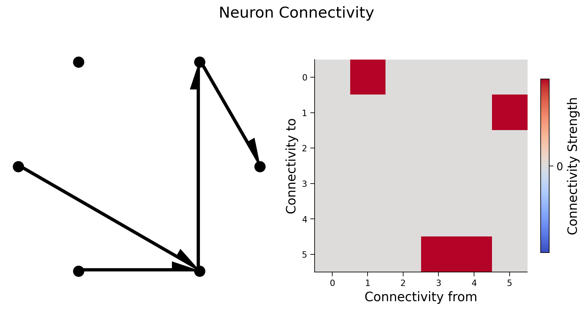
We will create the true connectivity matrix between 6 neurons and visualize it in two different ways: as a graph with directional edges between connected neurons and as an image of the connectivity matrix.

Check your understanding: do you understand how the left plot relates to the right plot below?

Execute this cell to get helper function create_connectivity and visualize connectivity

../../../_images/666241afe8c04cc4efe05b7fae31010ab22bf3b2b1321581c1c020370ba80bf3.png

Coding Exercise 2: System simulation#

In this exercise we’re going to simulate the system. Please complete the following function so that at every timestep the activity vector \(x\) is updated according to:

(454)#\[\begin{equation} \vec{x}_{t+1} = \sigma(A\vec{x}_t + \epsilon_t). \end{equation}\]

We will use helper function sigmoid, defined in the cell below.

Execute to enable helper function sigmoid

def simulate_neurons(A, timesteps, random_state=42):
  """Simulates a dynamical system for the specified number of neurons and timesteps.

  Args:
    A (np.array): the connectivity matrix
    timesteps (int): the number of timesteps to simulate our system.
    random_state (int): random seed for reproducibility

  Returns:
    - X has shape (n_neurons, timeteps). A schematic:
                ___t____t+1___
    neuron  0  |   0    1     |
              |   1    0     |
    neuron  i  |   0 -> 1     |
              |   0    0     |
              |___1____0_____|
  """
  np.random.seed(random_state)

  n_neurons = len(A)
  X = np.zeros((n_neurons, timesteps))

  for t in range(timesteps - 1):

    # Create noise vector
    epsilon = np.random.multivariate_normal(np.zeros(n_neurons), np.eye(n_neurons))

    ########################################################################
    ## TODO: Fill in the update rule for our dynamical system.
    ## Fill in function and remove
    raise NotImplementedError("Complete simulate_neurons")
    ########################################################################

    # Update activity vector for next step
    X[:, t + 1] = sigmoid(...)  # we are using helper function sigmoid

  return X


# Set simulation length
timesteps = 5000

# Simulate our dynamical system
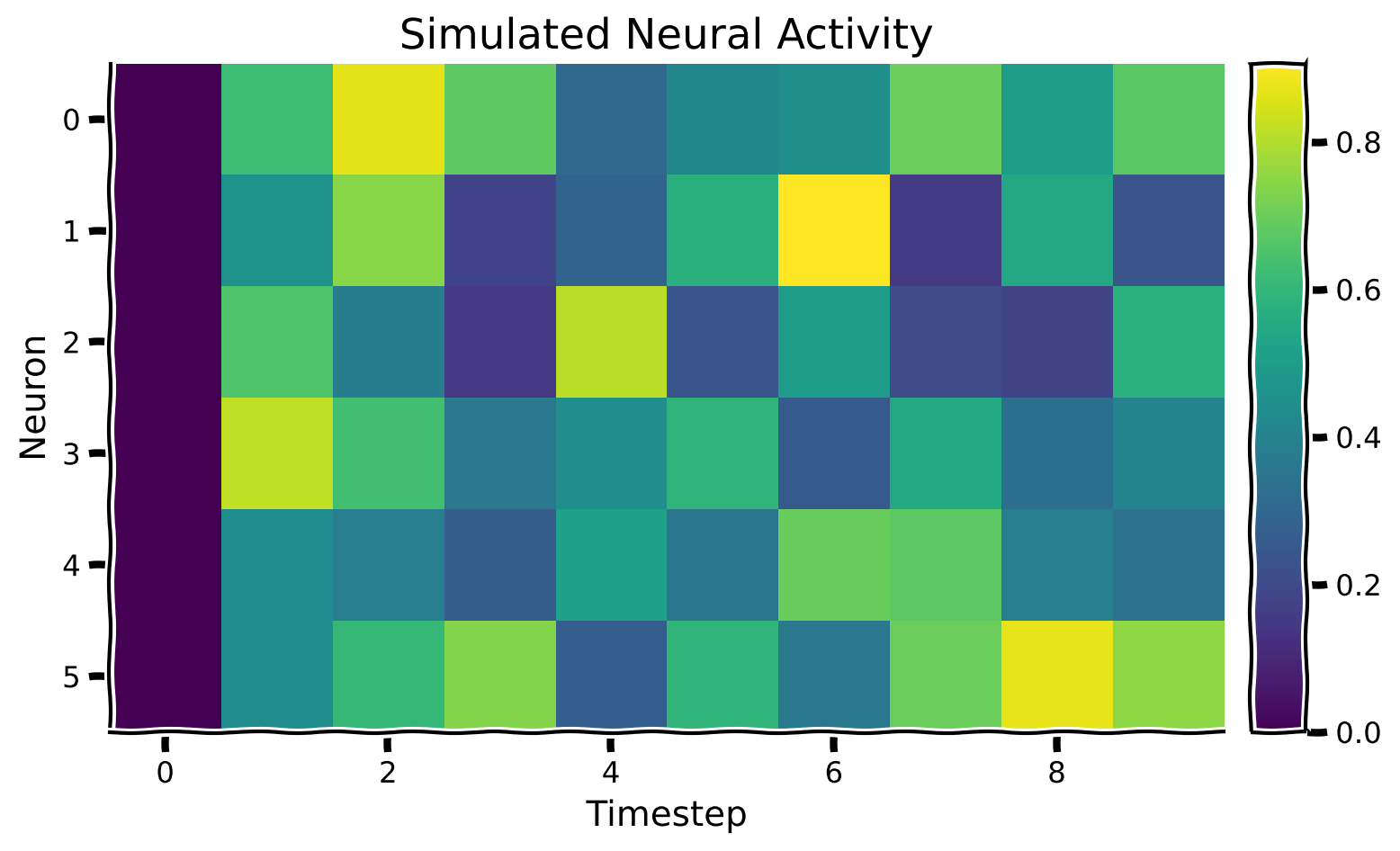
X = simulate_neurons(A, timesteps)

# Visualize
plot_neural_activity(X)

Click for solution

Example output:

Submit your feedback#

Section 3: Recovering connectivity through perturbation#

Estimated timing to here from start of tutorial: 22 min

Video 3: Perturbing systems#

Submit your feedback#

Section 3.1: Random perturbation in our system of neurons#

We want to get the causal effect of each neuron upon each other neuron. The ground truth of the causal effects is the connectivity matrix \(A\).

Remember that we would like to calculate:

(455)#\[\begin{equation} \delta_{A\to B} = \mathbb{E}[B | A=1] - \mathbb{E}[B | A=0] \end{equation}\]

We’ll do this by randomly setting the system state to 0 or 1 and observing the outcome after one timestep. If we do this \(N\) times, the effect of neuron \(i\) upon neuron \(j\) is:

(456)#\[\begin{equation} \delta_{x^i\to x^j} \approx \frac1N \sum_{\substack{t=0, \ t \text{ even}}}^N[x_{t+1}^j | x^i_t=1] - \frac1N \sum_{\substack{t=0, \ t \text{ even}}}^N[x_{t+1}^j | x^i_t=0] \end{equation}\]

This is just the average difference of the activity of neuron \(j\) in the two conditions.

We are going to calculate the above equation, but imagine it like intervening in activity every other timestep.

We will use helper function simulate_neurons_perturb. While the rest of the function is the same as the simulate_neurons function in the previous exercise, every time step we now additionally include:

if t % 2 == 0:
    X[:,t] = np.random.choice([0,1], size=n_neurons)

This means that at every other timestep, every neuron’s activity is changed to either 0 or 1.

Pretty serious perturbation, huh? You don’t want that going on in your brain.

Now visually compare the dynamics: Run this next cell and see if you can spot how the dynamics have changed.

Execute this cell to visualize perturbed dynamics

Section 3.2: Recovering connectivity from perturbed dynamics#

Video 4: Calculating causality#

Submit your feedback#

Coding Exercise 3.2: Using perturbed dynamics to recover connectivity#

From the above perturbed dynamics, write a function that recovers the causal effect of a given single neuron (selected_neuron) upon all other neurons in the system. Remember from above you’re calculating:

(457)#\[\begin{equation} \delta_{x^i\to x^j} \approx \frac1N \sum_{\substack{t=0, \ t \text{ even}}}^N[x_{t+1}^j | x^i_t=1] - \frac1N \sum_{\substack{t=0, \ t \text{ even}}}^N[x_{t+1}^j | x^i_t=0] \end{equation}\]

Recall that we perturbed every neuron at every other timestep. Despite perturbing every neuron, in this exercise we are concentrating on computing the causal effect of a single neuron (we will look at all neurons effects on all neurons next). We want to exclusively use the timesteps without perturbation for \(x^j_{t+1}\) and the timesteps with perturbation for \(x^j_{t}\) in the formulas above. In numpy, indexing occurs as array[ start_index : end_index : count_by]. So getting every other element in an array (such as every other timestep) is as easy as array[::2].

def get_perturbed_connectivity_from_single_neuron(perturbed_X, selected_neuron):
  """
  Computes the connectivity matrix from the selected neuron using differences in means.

  Args:
    perturbed_X (np.ndarray): the perturbed dynamical system matrix of shape
                              (n_neurons, timesteps)
    selected_neuron (int): the index of the neuron we want to estimate connectivity for

  Returns:
      estimated_connectivity (np.ndarray): estimated connectivity for the selected neuron,
                                           of shape (n_neurons,)
  """
  # Extract the perturbations of neuron 1 (every other timestep)
  neuron_perturbations = perturbed_X[selected_neuron, ::2]

  # Extract the observed outcomes of all the neurons (every other timestep)
  all_neuron_output = perturbed_X[:, 1::2]

  # Initialize estimated connectivity matrix
  estimated_connectivity = np.zeros(n_neurons)

  # Loop over neurons
  for neuron_idx in range(n_neurons):

    # Get this output neurons (neuron_idx) activity
    this_neuron_output = all_neuron_output[neuron_idx, :]

    # Get timesteps where the selected neuron == 0 vs == 1
    one_idx = np.argwhere(neuron_perturbations == 1)
    zero_idx = np.argwhere(neuron_perturbations == 0)

    ########################################################################
    ## TODO: Insert your code here to compute the neuron activation from perturbations.
    # Fill out function and remove
    raise NotImplementedError("Complete the function get_perturbed_connectivity_single_neuron")
    ########################################################################

    difference_in_means = ...

    estimated_connectivity[neuron_idx] = difference_in_means

  return estimated_connectivity


# Initialize the system
n_neurons = 6
timesteps = 5000
selected_neuron = 1

# Simulate our perturbed dynamical system
perturbed_X = simulate_neurons_perturb(A, timesteps)

# Measure connectivity of neuron 1
estimated_connectivity = get_perturbed_connectivity_from_single_neuron(perturbed_X, selected_neuron)
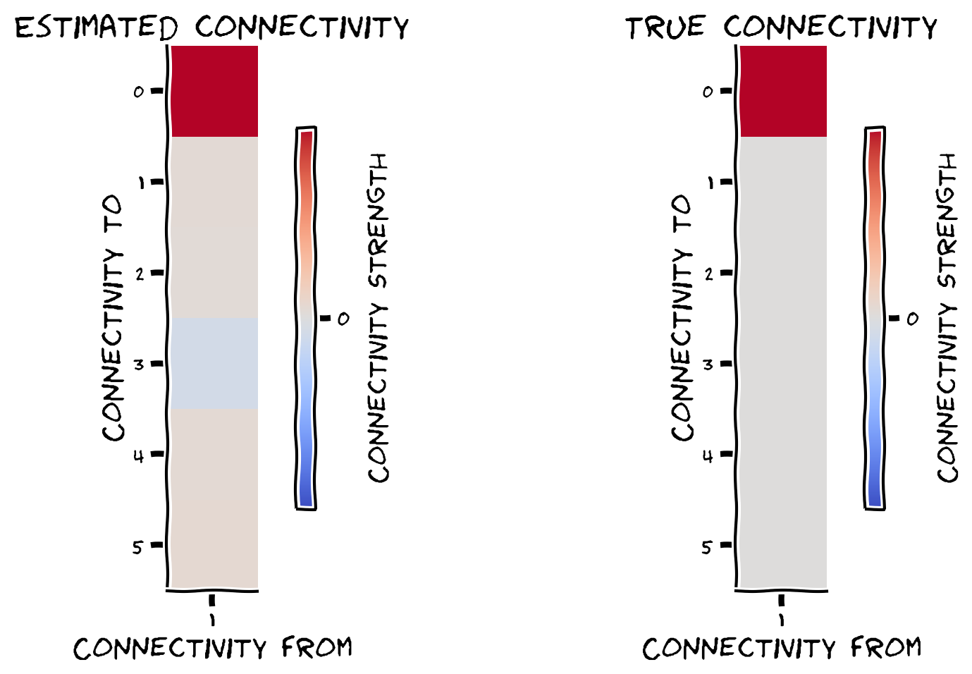
plot_true_vs_estimated_connectivity(estimated_connectivity, A, selected_neuron)

Click for solution

Example output:

Submit your feedback#

We can quantify how close our estimated connectivity matrix is to our true connectivity matrix by correlating them. We should see almost perfect correlation between our estimates and the true connectivity - do we?

# Correlate true vs estimated connectivity matrix
print(np.corrcoef(A[:, selected_neuron], estimated_connectivity)[1, 0])

Note on interpreting A: Strictly speaking, \(A\) is not the matrix of causal effects but rather the dynamics matrix. So why compare them like this? The answer is that \(A\) and the effect matrix both are \(0\) everywhere except where there is a directed connection. So they should have a correlation of \(1\) if we estimate the effects correctly. (Their scales, however, are different. This is in part because the nonlinearity \(\sigma\) squashes the values of \(x\) to \([0,1]\).) See the Appendix after Tutorial 2 for more discussion of using correlation as a metric.

Nice job! You just estimated connectivity for a single neuron.

We’re now going to use the same strategy for all neurons at once. We provide this helper function get_perturbed_connectivity_all_neurons. If you’re curious about how this works and have extra time, check out Bonus Section 1.

Execute to get helper function get_perturbed_connectivity_all_neurons

Execute this cell to visualize true vs estimated connectivity

../../../_images/98c3803f14e6b5280f161e001532e6fa4f3861b2232df50bf468b6df3ac76c02.png

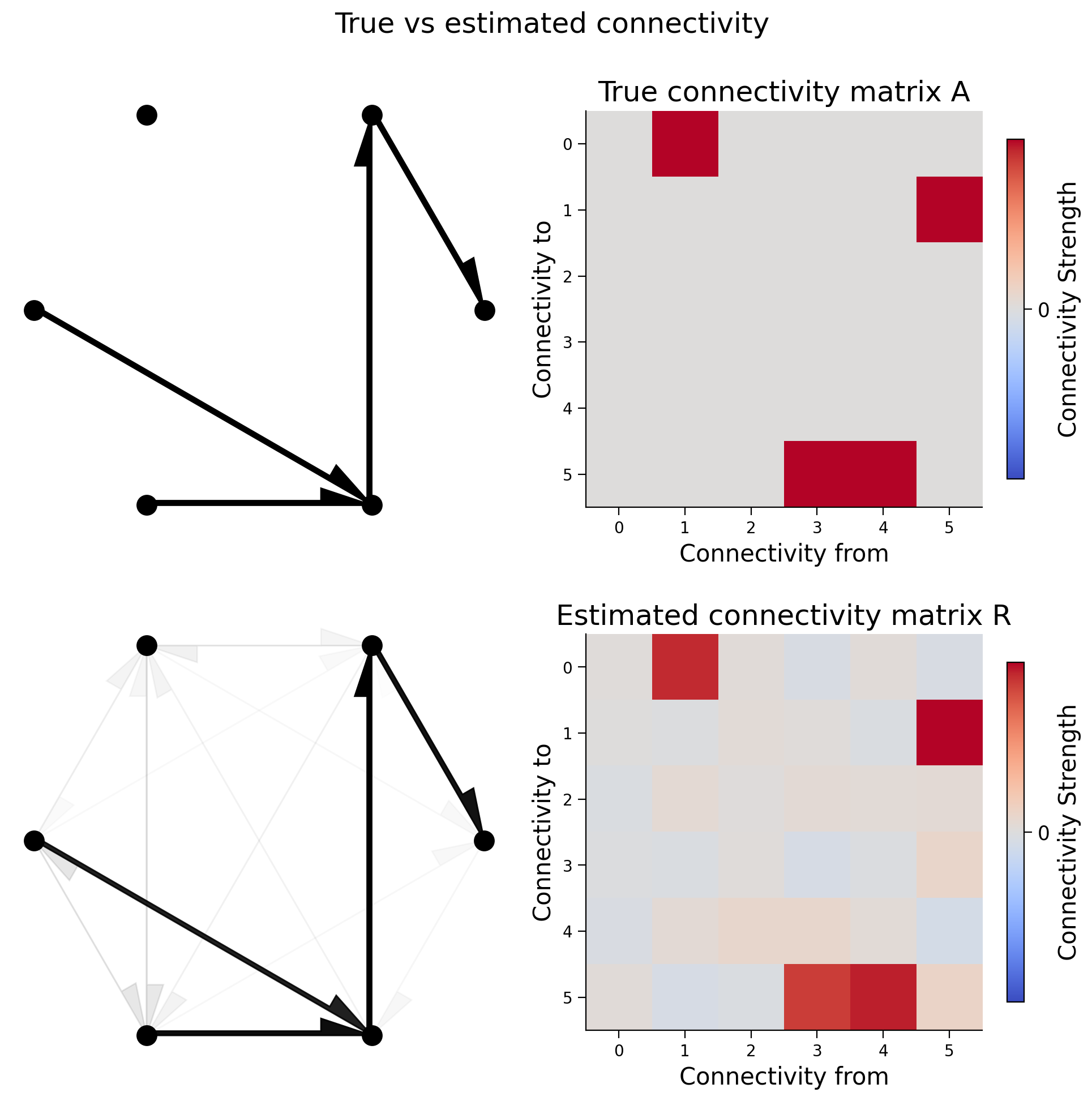
We can again calculate the correlation coefficient between the elements of the two matrices. In the cell below, we compute the correlation coefficient between true and estimated connectivity matrices. It is almost 1 so we do a good job recovering the true causality of the system!

print(np.corrcoef(A.transpose().flatten(), R.flatten())[1, 0])

0.987593404378358

Summary#

Estimated timing of tutorial: 40 min

Video 5: Summary#

Submit your feedback#

In this tutorial, we learned about how to define and estimate causality using perturbations. In particular we:

Learned how to simulate a system of connected neurons
Learned how to estimate the connectivity between neurons by directly perturbing neural activity

If you are interested in causality after NMA ends, here are some useful texts to consult.

Causal Inference for Statistics, Social, and Biomedical Sciences by Imbens and Rubin
Causal Inference: What If by Hernan and Rubin
Mostly Harmless Econometrics by Angrist and Pischke
See here for an application to neuroscience

Bonus#

Bonus Section 1: Computation of the estimated connectivity matrix#

This is an explanation of what the code is doing in get_perturbed_connectivity_all_neurons()

First, we compute an estimated connectivity matrix \(R\). We extract perturbation matrix \(P\) and outcomes matrix \(O\):

(458)#\[\begin{equation} P = \begin{bmatrix} \mid & \mid & ... & \mid \\ x_0 & x_2 & ... & x_T \\ \mid & \mid & ... & \mid \end{bmatrix}_{n \times T/2} \end{equation}\]

(459)#\[\begin{equation} O = \begin{bmatrix} \mid & \mid & ... & \mid \\ x_1 & x_3 & ... & x_{T-1} \\ \mid & \mid & ... & \mid \end{bmatrix}_{n \times T/2} \end{equation}\]

And calculate the correlation of matrix \(S\), which is \(P\) and \(O\) stacked on each other:

(460)#\[\begin{equation} S = \begin{bmatrix} P \\ O \end{bmatrix}_{2n \times T/2} \end{equation}\]

We then extract \(R\) as the upper right \(n \times n\) block of \( \text{corr}(S)\):

This is because the upper right block corresponds to the estimated perturbation effect on outcomes for each pair of neurons in our system.

This method gives an estimated connectivity matrix that is the proportional to the result you would obtain with differences in means, and differs only in a proportionality constant that depends on the variance of \(x\).

Tutorial 1: Interventions

Contents

Tutorial 1: Interventions#

Tutorial Objectives#

Setup#

Install and import feedback gadget#

Figure Settings#

Plotting Functions#

Section 1: Defining and estimating causality#

Video 1: Defining causality#

Submit your feedback#

Coding Exercise 1: Randomized controlled trial for two neurons#

Submit your feedback#

Section 2: Simulating a system of neurons#

Video 2: Simulated neural system model#

Submit your feedback#

Coding Exercise 2: System simulation#

Submit your feedback#

Section 3: Recovering connectivity through perturbation#

Video 3: Perturbing systems#

Submit your feedback#

Section 3.1: Random perturbation in our system of neurons#

Section 3.2: Recovering connectivity from perturbed dynamics#

Video 4: Calculating causality#

Submit your feedback#

Coding Exercise 3.2: Using perturbed dynamics to recover connectivity#

Submit your feedback#

Summary#

Video 5: Summary#

Submit your feedback#

Bonus#

Bonus Section 1: Computation of the estimated connectivity matrix#