![]()

Tutorial 2: Differential Equations#
Week 0, Day 4: Calculus
By Neuromatch Academy
Content creators: John S Butler, Arvind Kumar with help from Rebecca Brady
Content reviewers: Swapnil Kumar, Sirisha Sripada, Matthew McCann, Tessy Tom
Production editors: Matthew McCann, Ella Batty
Tutorial Objectives#
Estimated timing of tutorial: 45 minutes
A great deal of neuroscience can be modeled using differential equations, from gating channels to single neurons to a network of neurons to blood flow to behavior. A simple way to think about differential equations is they are equations that describe how something changes.
The most famous of these in neuroscience is the Nobel Prize-winning Hodgkin-Huxley equation, which describes a neuron by modeling the gating of each axon. But we will not start there; we will start a few steps back.
Differential Equations are mathematical equations that describe how something like a population or a neuron changes over time. Differential equations are so useful because they can generalize a process such that one equation can be used to describe many different outcomes. The general form of a first-order differential equation is:
which can be read as “the change in a process \(y\) over time \(t\) is a function \(f\) of time \(t\) and itself \(y\)”. This might initially seem like a paradox as you are using a process \(y\) you want to know about to describe itself, a bit like the MC Escher drawing of two hands painting each other. But that is the beauty of mathematics - this can be solved sometimes, and when it cannot be solved exactly, we can use numerical methods to estimate the answer (as we will see in the next tutorial).
In this tutorial, we will see how differential equations are motivated by observations of physical responses. We will break down the population differential equation, then the integrate and fire model, which leads nicely into raster plots and frequency-current curves to rate models.
Steps:
Get an intuitive understanding of a linear population differential equation (humans, not neurons)
Visualize the relationship between the change in population and the population
Breakdown the Leaky Integrate and Fire (LIF) differential equation
Code the exact solution of a LIF for a constant input
Visualize and listen to the response of the LIF for different inputs
Setup#
Install and import feedback gadget#
Show code cell source
# @title Install and import feedback gadget

!pip3 install vibecheck datatops --quiet

from vibecheck import DatatopsContentReviewContainer
def content_review(notebook_section: str):
    return DatatopsContentReviewContainer(
        "",  # No text prompt
        notebook_section,
        {
            "url": "https://pmyvdlilci.execute-api.us-east-1.amazonaws.com/klab",
            "name": "neuromatch-precourse",
            "user_key": "8zxfvwxw",
        },
    ).render()


feedback_prefix = "W0D4_T2"
# Imports
import numpy as np
import matplotlib.pyplot as plt
Figure Settings#
Show code cell source
# @title Figure Settings
import logging
logging.getLogger('matplotlib.font_manager').disabled = True
import IPython.display as ipd
from matplotlib import gridspec
import ipywidgets as widgets  # interactive display
%config InlineBackend.figure_format = 'retina'
# use NMA plot style
plt.style.use("https://raw.githubusercontent.com/NeuromatchAcademy/content-creation/main/nma.mplstyle")
my_layout = widgets.Layout()
Plotting Functions#
Show code cell source
# @title Plotting Functions

def plot_dPdt(alpha=.3):
  """ Plots change in population over time
    Args:
      alpha: Birth Rate
    Returns:
      A figure two panel figure
      left panel: change in population as a function of population
      right panel: membrane potential as a function of time
  """

  with plt.xkcd():
    time=np.arange(0, 10 ,0.01)
    fig = plt.figure(figsize=(12,4))
    gs = gridspec.GridSpec(1, 2)

    ## dpdt as a fucntion of p
    plt.subplot(gs[0])
    plt.plot(np.exp(alpha*time), alpha*np.exp(alpha*time))
    plt.xlabel(r'Population $p(t)$ (millions)')
    plt.ylabel(r'$\frac{d}{dt}p(t)=\alpha p(t)$')

    ## p exact solution
    plt.subplot(gs[1])
    plt.plot(time, np.exp(alpha*time))
    plt.ylabel(r'Population $p(t)$ (millions)')
    plt.xlabel('time (years)')
    plt.show()


def plot_V_no_input(V_reset=-75):
  """
    Args:
      V_reset: Reset Potential
    Returns:
      A figure two panel figure
      left panel: change in membrane potential as a function of membrane potential
      right panel: membrane potential as a function of time
  """
  E_L=-75
  tau_m=10
  t=np.arange(0,100,0.01)
  V= E_L+(V_reset-E_L)*np.exp(-(t)/tau_m)
  V_range=np.arange(-90,0,1)
  dVdt=-(V_range-E_L)/tau_m

  with plt.xkcd():
    time=np.arange(0, 10, 0.01)
    fig = plt.figure(figsize=(12, 4))
    gs = gridspec.GridSpec(1, 2)

    plt.subplot(gs[0])
    plt.plot(V_range,dVdt)
    plt.hlines(0,min(V_range),max(V_range), colors='black', linestyles='dashed')
    plt.vlines(-75, min(dVdt), max(dVdt), colors='black', linestyles='dashed')
    plt.plot(V_reset,-(V_reset - E_L)/tau_m, 'o', label=r'$V_{reset}$')
    plt.text(-50, 1, 'Positive')
    plt.text(-50, -2, 'Negative')
    plt.text(E_L - 1, max(dVdt), r'$E_L$')
    plt.legend()
    plt.xlabel('Membrane Potential V (mV)')
    plt.ylabel(r'$\frac{dV}{dt}=\frac{-(V(t)-E_L)}{\tau_m}$')

    plt.subplot(gs[1])
    plt.plot(t,V)
    plt.plot(t[0],V_reset,'o')
    plt.ylabel(r'Membrane Potential $V(t)$ (mV)')
    plt.xlabel('time (ms)')
    plt.ylim([-95, -60])

    plt.show()


## LIF PLOT
def plot_IF(t, V,I,Spike_time):
  """
    Args:
      t  : time
      V  : membrane Voltage
      I  : Input
      Spike_time : Spike_times
    Returns:
      figure with three panels
      top panel: Input as a function of time
      middle panel: membrane potential as a function of time
      bottom panel: Raster plot
  """

  with plt.xkcd():
    fig = plt.figure(figsize=(12, 4))
    gs = gridspec.GridSpec(3, 1,  height_ratios=[1, 4, 1])

    # PLOT OF INPUT
    plt.subplot(gs[0])
    plt.ylabel(r'$I_e(nA)$')
    plt.yticks(rotation=45)
    plt.hlines(I,min(t),max(t),'g')
    plt.ylim((2, 4))
    plt.xlim((-50, 1000))

    # PLOT OF ACTIVITY
    plt.subplot(gs[1])
    plt.plot(t,V)
    plt.xlim((-50, 1000))
    plt.ylabel(r'$V(t)$(mV)')

    # PLOT OF SPIKES
    plt.subplot(gs[2])
    plt.ylabel(r'Spike')
    plt.yticks([])
    plt.scatter(Spike_time, 1 * np.ones(len(Spike_time)), color="grey", marker=".")
    plt.xlim((-50, 1000))
    plt.xlabel('time(ms)')
    plt.show()


## Plotting the differential Equation
def plot_dVdt(I=0):
  """
    Args:
      I  : Input Current
    Returns:
      figure of change in membrane potential as a function of membrane potential
  """

  with plt.xkcd():
    E_L = -75
    tau_m = 10
    V = np.arange(-85, 0, 1)
    g_L = 10.
    fig = plt.figure(figsize=(6, 4))

    plt.plot(V,(-(V-E_L) + I*10) / tau_m)
    plt.hlines(0, min(V), max(V), colors='black', linestyles='dashed')
    plt.xlabel('V (mV)')
    plt.ylabel(r'$\frac{dV}{dt}$')
    plt.show()
Helper Functions#
Show code cell source
# @title Helper Functions

## EXACT SOLUTION OF LIF
def Exact_Integrate_and_Fire(I,t):
  """
    Args:
      I  : Input Current
      t : time
    Returns:
      Spike : Spike Count
      Spike_time : Spike time
      V_exact : Exact membrane potential
  """

  Spike = 0
  tau_m = 10
  R = 10
  t_isi = 0
  V_reset = E_L = -75
  V_exact = V_reset * np.ones(len(t))
  V_th = -50
  Spike_time = []

  for i in range(0, len(t)):

    V_exact[i] = E_L + R*I + (V_reset - E_L - R*I) * np.exp(-(t[i]-t_isi)/tau_m)

    # Threshold Reset
    if V_exact[i] > V_th:
        V_exact[i-1] = 0
        V_exact[i] = V_reset
        t_isi = t[i]
        Spike = Spike+1
        Spike_time = np.append(Spike_time, t[i])

  return Spike, Spike_time, V_exact
Section 0: Introduction#
Video 1: Why do we care about differential equations?#
Submit your feedback#
Show code cell source
# @title Submit your feedback
content_review(f"{feedback_prefix}_Why_do_we_care_about_differential_equations_Video")
Section 1: Population differential equation#
Video 2: Population differential equation#
Submit your feedback#
Show code cell source
# @title Submit your feedback
content_review(f"{feedback_prefix}_Population_differential_equation_Video")
This video covers our first example of a differential equation: a differential equation which models the change in population.
Click here for text recap of video
To get an intuitive feel of a differential equations, we will start with a population differential equation, which models the change in population [1], that is human population not neurons, we will get to neurons later. Mathematically it is written like:
where \(p(t)\) is the population of the world and \(\alpha\) is a parameter representing birth rate.
Another way of thinking about the models is that the equation
The equation is saying something reasonable maybe not the perfect model but a good start.
Think! 1.1: Interpretating the behavior of a linear population equation#
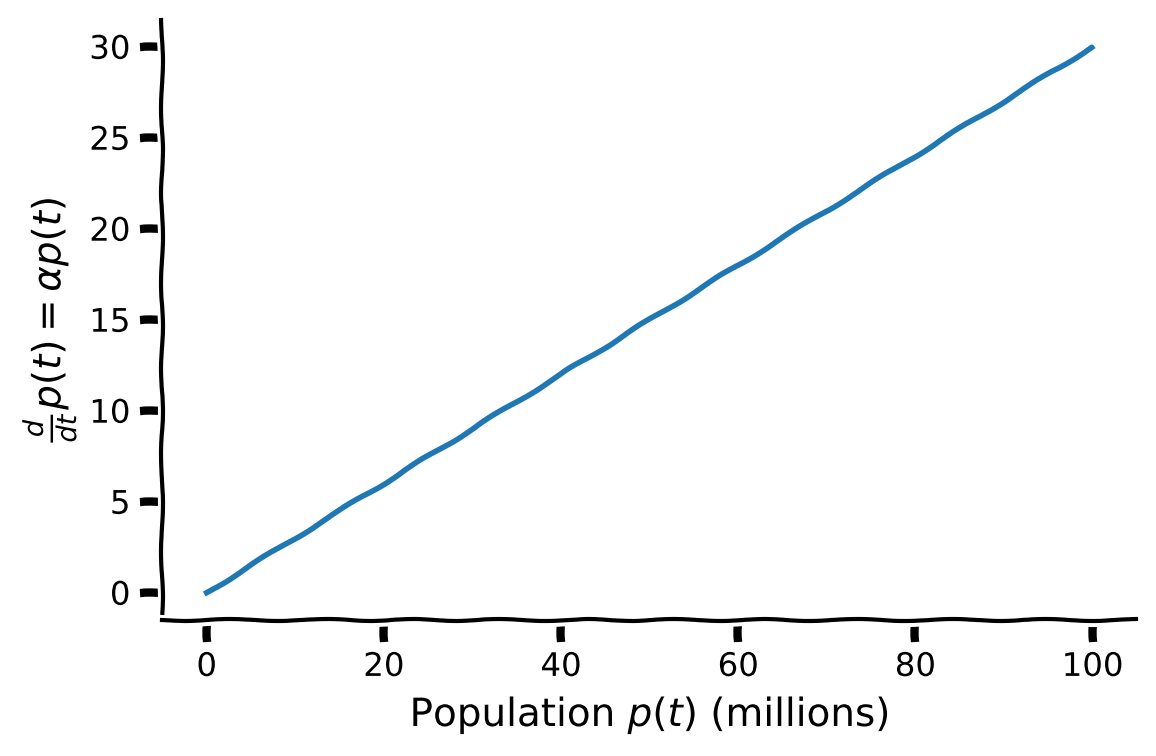
Using the plot below of change of population \(\frac{d}{dt} p(t) \) as a function of population \(p(t)\) with birth-rate \(\alpha=0.3\), discuss the following questions:
Why is the population differential equation known as a linear differential equation?
How does population size affect the rate of change of the population?
Execute the code to plot the rate of change of population as a function of population
Show code cell source
# @markdown Execute the code to plot the rate of change of population as a function of population
p = np.arange(0, 100, 0.1)

with plt.xkcd():

  dpdt = 0.3*p
  fig = plt.figure(figsize=(6, 4))
  plt.plot(p, dpdt)
  plt.xlabel(r'Population $p(t)$ (millions)')
  plt.ylabel(r'$\frac{d}{dt}p(t)=\alpha p(t)$')
  plt.show()
Submit your feedback#
Show code cell source
# @title Submit your feedback
content_review(f"{feedback_prefix}_Interpretating_the_behavior_of_a_linear_population_equation_Discussion")
Section 1.1: Exact solution of the population equation#
Section 1.1.1: Initial condition#
The linear population differential equation is an initial value differential equation because we need an initial population value to solve it. Here we will set our initial population at time \(0\) to \(1\):
Different initial conditions will lead to different answers but will not change the differential equation. This is one of the strengths of a differential equation.
Section 1.1.2: Exact Solution#
To calculate the exact solution of a differential equation, we must integrate both sides. Instead of numerical integration (as you delved into in the last tutorial), we will first try to solve the differential equations using analytical integration. As with derivatives, we can find analytical integrals of simple equations by consulting a list. We can then get integrals for more complex equations using some mathematical tricks - the harder the equation, the more obscure the trick.
The linear population equation
has the exact solution:
The exact solution written in words is:
Most differential equations do not have a known exact solution, so we will show how the solution can be estimated in the next tutorial on numerical methods.
A small aside: a good deal of progress in mathematics was due to mathematicians writing taunting letters to each other, saying they had a trick to solve something better than everyone else. So do not worry too much about the tricks.
Example Exact Solution of the Population Equation#
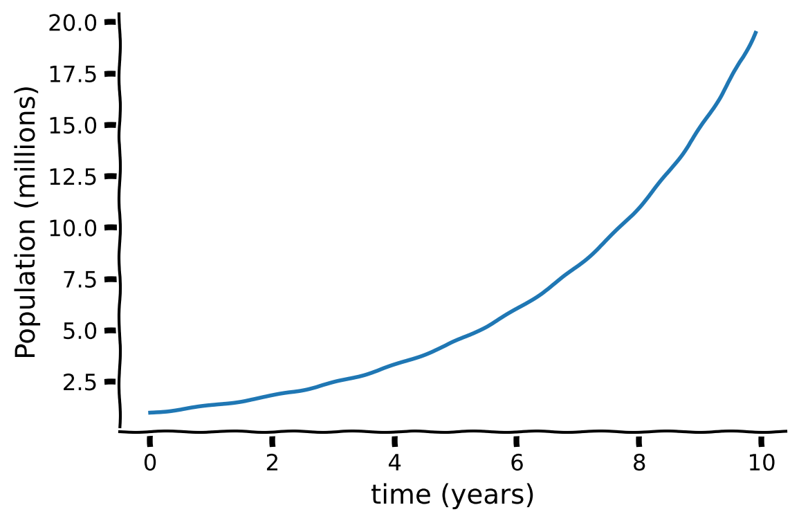
Let’s consider the population differential equation with a birth rate \(\alpha=0.3\):
with the initial condition
It has an exact solution
Execute code to plot the exact solution
Show code cell source
# @markdown Execute code to plot the exact solution
t = np.arange(0, 10, 0.1) # Time from 0 to 10 years in 0.1 steps

with plt.xkcd():

  p = np.exp(0.3 * t)

  fig = plt.figure(figsize=(6, 4))
  plt.plot(t, p)
  plt.ylabel('Population (millions)')
  plt.xlabel('time (years)')
  plt.show()
Section 1.2: Parameters of the differential equation#
Estimated timing to here from start of tutorial: 12 min
One of the goals when designing a differential equation is to make it generalizable. This means that the differential equation will give reasonable solutions for different countries with different birth rates \(\alpha\).
Interactive Demo 1.2: Parameter Change#
Play with the widget to see the relationship between \(\alpha\) and the population differential equation as a function of population (left-hand side) and the population solution as a function of time (right-hand side). Pay close attention to the transition point from positive to negative.
How do changing parameters of the population equation affect the outcome?
What happens when \(\alpha < 0\)?
What happens when \(\alpha > 0\)?
What happens when \(\alpha = 0\)?
Make sure you execute this cell to enable the widget!
Show code cell source
# @markdown Make sure you execute this cell to enable the widget!
my_layout.width = '450px'
@widgets.interact(
    alpha=widgets.FloatSlider(.3, min=-1., max=1., step=.1, layout=my_layout)
)
def Pop_widget(alpha):
  plot_dPdt(alpha=alpha)
  plt.show()
Submit your feedback#
Show code cell source
# @title Submit your feedback
content_review(f"{feedback_prefix}_Parameter_change_Interactive_Demo")
The population differential equation is an over-simplification and has some pronounced limitations:
Population growth is not exponential as there are limited resources, so the population will level out at some point.
It does not include any external factors on the populations, like weather, predators, and prey.
These kinds of limitations can be addressed by extending the model.
While it might not seem that the population equation has direct relevance to neuroscience, a similar equation is used to describe the accumulation of evidence for decision-making. This is known as the Drift Diffusion Model, and you will see it in more detail in the Linear System Day in Neuromatch (W2D2).
Another differential equation similar to the population equation is the Leaky Integrate and Fire model, which you may have seen in the Python pre-course materials on W0D1 and W0D2. It will turn up later in Neuromatch as well. Below we will delve into the motivation of the differential equation.
Section 2: The leaky integrate and fire (LIF) model#
Video 3: The leaky integrate and fire model#
Submit your feedback#
Show code cell source
# @title Submit your feedback
content_review(f"{feedback_prefix}_The_leaky_integrate_and_fire_model_Video")
This video covers the Leaky Integrate and Fire model (a linear differential equation which describes the membrane potential of a single neuron).
Click here for text recap of full LIF equation from video
The Leaky Integrate and Fire Model is a linear differential equation that describes the membrane potential (\(V\)) of a single neuron which was proposed by Louis Édouard Lapicque in 1907 [2].
The subthreshold membrane potential dynamics of a LIF neuron is described by
where \(\tau_m\) is the time constant, \(V\) is the membrane potential, \(E_L\) is the resting potential, \(R_m\) is membrane resistance, and \(I\) is the external input current.
In the next few sections, we will break down the full LIF equation and then build it back up to get an intuitive feel of the different facets of the differential equation.
Section 2.1: LIF without input#
Estimated timing to here from start of tutorial: 18 min
As seen in the video, we will first model an LIF neuron without input, which results in the equation:
where \(\tau_m\) is the time constant, \(V\) is the membrane potential, and \(E_L\) is the resting potential.
Click here for further details (from video)
Removing the input gives the equation
which can be written in words as:
The equation can be re-arranged to look even more like the population equation:
Think! 2.1: Effect of membrane potential \(V\) on the LIF model#
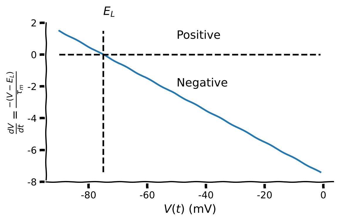
The plot the below shows the change in membrane potential \(\frac{dV}{dt}\) as a function of membrane potential \(V\) with the parameters set as:
E_L = -75V_reset = -50tau_m = 10.
What is the effect on \(\frac{dV}{dt}\) when \(V>-75\) mV?
What is the effect on \(\frac{dV}{dt}\) when \(V<-75\) mV
What is the effect on \(\frac{dV}{dt}\) when \(V=-75\) mV?
Make sure you execute this cell to plot the relationship between dV/dt and V
Show code cell source
# @markdown Make sure you execute this cell to plot the relationship between dV/dt and V
# Parameter definition
E_L = -75
tau_m = 10

# Range of Values of V
V = np.arange(-90, 0, 1)
dV = -(V - E_L) / tau_m

with plt.xkcd():

  fig = plt.figure(figsize=(6, 4))
  plt.plot(V, dV)
  plt.hlines(0, min(V), max(V), colors='black', linestyles='dashed')
  plt.vlines(-75, min(dV), max(dV), colors='black', linestyles='dashed')

  plt.text(-50, 1, 'Positive')
  plt.text(-50, -2, 'Negative')
  plt.text(E_L, max(dV) + 1, r'$E_L$')
  plt.xlabel(r'$V(t)$ (mV)')
  plt.ylabel(r'$\frac{dV}{dt}=\frac{-(V-E_L)}{\tau_m}$')
  plt.ylim(-8, 2)
  plt.show()
Submit your feedback#
Show code cell source
# @title Submit your feedback
content_review(f"{feedback_prefix}_Effect_of_membrane_potential_Interactive_Demo")
Section 2.1.1: Exact Solution of the LIF model without input#
The LIF model has the exact solution:
where \(\tau_m\) is the time constant, \(V\) is the membrane potential, \(E_L\) is the resting potential, and \(V_{reset}\) is the initial membrane potential.
Click here for further details (from video)
Similar to the population equation, we need an initial membrane potential at time \(0\) to solve the LIF model.
With this equation
where is \(V_{reset}\) is called the reset potential.
The LIF model has the exact solution:
Interactive Demo 2.1.1: Initial Condition \(V_{reset}\)#
This exercise is to get an intuitive feel of how the different initial conditions \(V_{reset}\) impact the differential equation of the LIF and the exact solution for the equation:
with the parameters set as:
E_L = -75,tau_m = 10.
The panel on the left-hand side plots the change in membrane potential \(\frac{dV}{dt}\) as a function of membrane potential \(V\) and the right-hand side panel plots the exact solution \(V\) as a function of time \(t,\) the green dot in both panels is the reset potential \(V_{reset}\).
Pay close attention to when \(V_{reset}=E_L=-75\)mV.
How does the solution look with initial values of \(V_{reset} < -75\)?
How does the solution look with initial values of \(V_{reset} > -75\)?
How does the solution look with initial values of \(V_{reset} = -75\)?
Make sure you execute this cell to enable the widget!
Show code cell source
#@markdown Make sure you execute this cell to enable the widget!
my_layout.width = '450px'
@widgets.interact(
  V_reset=widgets.FloatSlider(-77., min=-91., max=-61., step=2,
                              layout=my_layout)
)

def V_reset_widget(V_reset):
  plot_V_no_input(V_reset)
Submit your feedback#
Show code cell source
# @title Submit your feedback
content_review(f"{feedback_prefix}_Initial_condition_Vreset_Interactive_Demo")
Section 2.2: LIF with input#
Estimated timing to here from start of tutorial: 24 min
We will re-introduce the input \(I\) and membrane resistance \(R_m\) giving the original equation:
The input can be other neurons or sensory information.
Interactive Demo 2.2: The Impact of Input#
The interactive plot below manipulates \(I\) in the differential equation.
With increasing input, how does the \(\frac{dV}{dt}\) change? How would this impact the solution?
Make sure you execute this cell to enable the widget!
Show code cell source
# @markdown Make sure you execute this cell to enable the widget!
my_layout.width = '450px'
@widgets.interact(
  I=widgets.FloatSlider(3., min=0., max=20., step=2,
                                layout=my_layout)
)

def Pop_widget(I):
  plot_dVdt(I=I)
  plt.show()
Submit your feedback#
Show code cell source
# @title Submit your feedback
content_review(f"{feedback_prefix}_The_impact_of_Input_Interactive_Demo")
Section 2.2.1: LIF exact solution#
The LIF with a constant input has a known exact solution:
which is written as:
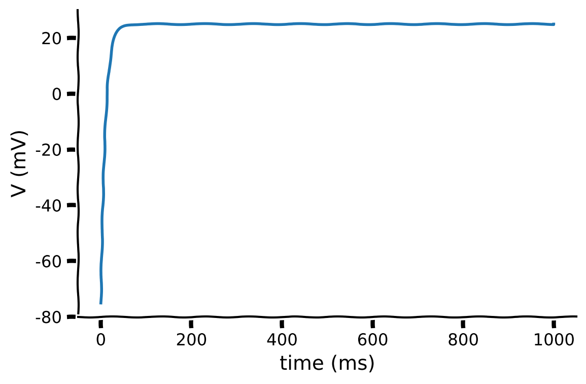
The plot below shows the exact solution of the membrane potential with the parameters set as:
V_reset = -75,E_L = -75,tau_m = 10,R_m = 10,I = 10.
Ask yourself, does the result make biological sense? If not, what would you change? We’ll delve into this in the next section
Make sure you execute this cell to see the exact solution
Show code cell source
# @markdown Make sure you execute this cell to see the exact solution
dt = 0.5
t_rest = 0

t = np.arange(0, 1000, dt)

tau_m = 10
R_m = 10
V_reset = E_L = -75

I = 10

V = E_L + R_m*I + (V_reset - E_L - R_m*I) * np.exp(-(t)/tau_m)

with plt.xkcd():

  fig = plt.figure(figsize=(6, 4))
  plt.plot(t,V)
  plt.ylabel('V (mV)')
  plt.xlabel('time (ms)')
  plt.show()
Section 2.3: Maths is one thing, but neuroscience matters#
Estimated timing to here from start of tutorial: 30 min
Video 4: Adding firing to the LIF#
Submit your feedback#
Show code cell source
# @title Submit your feedback
content_review(f"{feedback_prefix}_Adding_firing_to_the_LIF_Video")
This video first recaps the introduction of input to the leaky integrate and fire model and then delves into how we add spiking behavior (or firing) to the model.
Click here for text recap of video
While the mathematics of the exact solution is exact, it is not biologically valid as a neuron spikes and definitely does not plateau at a very positive value.
To model the firing of a spike, we must have a threshold voltage \(V_{th}\) such that if the voltage \(V(t)\) goes above it, the neuron spikes $\(V(t)>V_{th}.\)\( We must record the time of spike \)t_{isi}\( and count the number of spikes \)\(t_{isi}=t, \)\( \)\(𝑆𝑝𝑖𝑘𝑒=𝑆𝑝𝑖𝑘𝑒+1.\)\( Then reset the membrane voltage \)V(t)\( \)\(V(t_{isi} )=V_{Reset}.\)$
To take into account the spike the exact solution becomes:
while this does make the neuron spike, it introduces a discontinuity which is not as elegant mathematically as it could be, but it gets results so that is good.
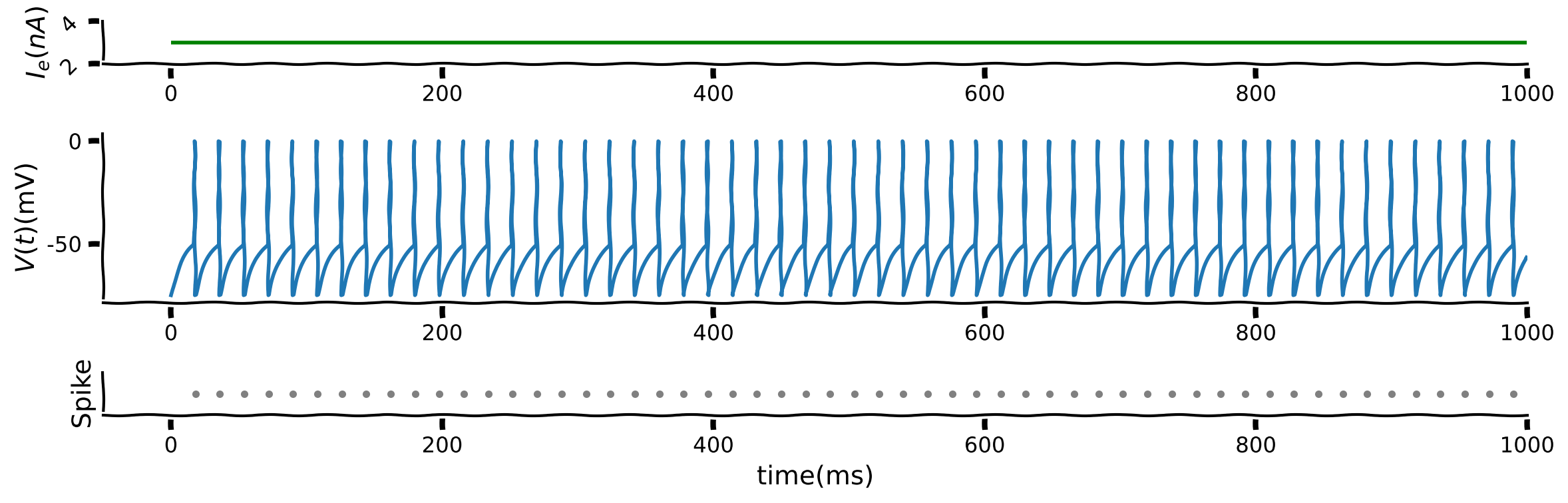
Interactive Demo 2.3.1: Input on spikes#
This exercise shows the relationship between the firing rate and the Input for the exact solution V of the LIF:
with the parameters set as:
V_reset = -75,E_L = -75,tau_m = 10,R_m = 10.
Below is a figure with three panels;
the top panel is the input, \(I,\)
the middle panel is the membrane potential \(V(t)\). To illustrate the spike, \(V(t)\) is set to \(0\) and then reset to \(-75\) mV when there is a spike.
the bottom panel is the raster plot with each dot indicating a spike.
First, as electrophysiologists normally listen to spikes when conducting experiments, listen to the music of the firing rate for a single value of \(I\).
Note: The audio doesn’t work in some browsers so don’t worry about it if you can’t hear anything.
Make sure you execute this cell to be able to hear the neuron
Show code cell source
# @markdown Make sure you execute this cell to be able to hear the neuron
I = 3
t = np.arange(0, 1000, dt)
Spike, Spike_time, V = Exact_Integrate_and_Fire(I, t)

plot_IF(t, V, I, Spike_time)
ipd.Audio(V, rate=len(V))
Manipulate the input into the LIF to see the impact of input on the firing pattern (rate).
What is the effect of \(I\) on spiking?
Is this biologically valid?
Make sure you execute this cell to enable the widget!
Show code cell source
# @markdown Make sure you execute this cell to enable the widget!
my_layout.width = '450px'
@widgets.interact(
  I=widgets.FloatSlider(3, min=2.0, max=4., step=.1,
                              layout=my_layout)
)

def Pop_widget(I):
  Spike, Spike_time, V = Exact_Integrate_and_Fire(I, t)
  plot_IF(t, V, I, Spike_time)
Submit your feedback#
Show code cell source
# @title Submit your feedback
content_review(f"{feedback_prefix}_Input_on_spikes_Interactive_Demo")
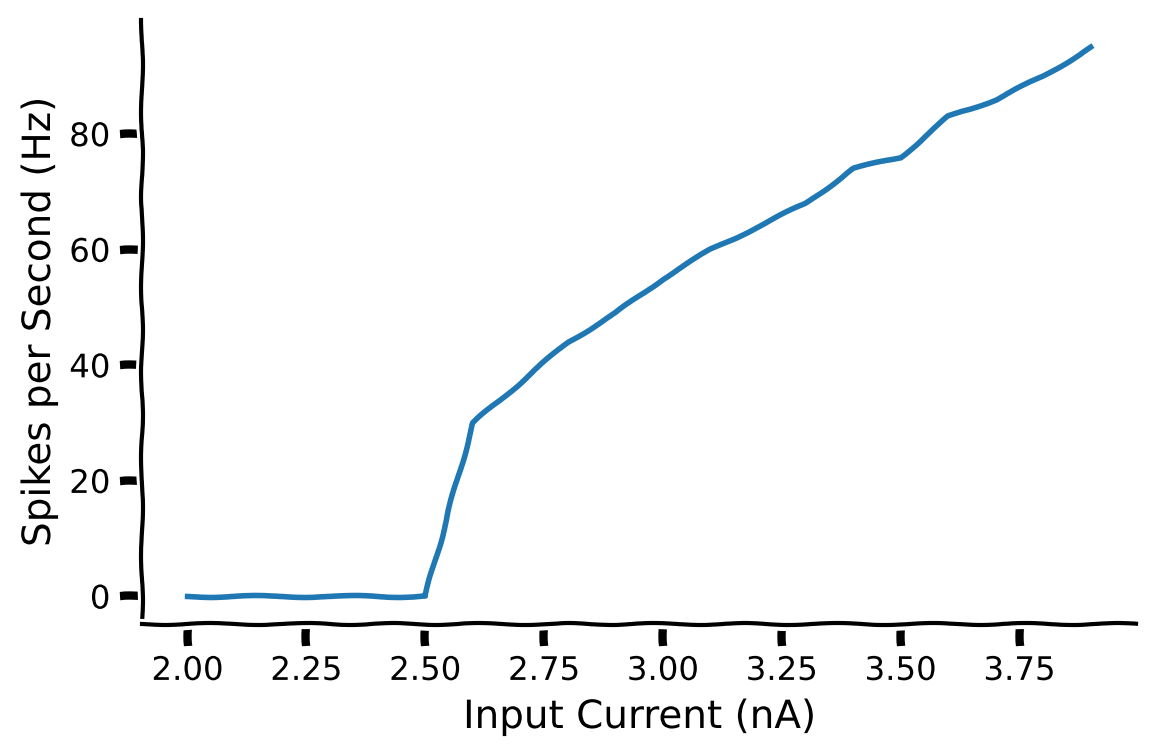
Section 2.4 Firing Rate as a function of Input#
Estimated timing to here from start of tutorial: 38 min
The firing frequency of a neuron plotted as a function of current is called an input-output curve (F–I curve). It is also known as a transfer function, which you came across in the previous tutorial. This function is one of the starting points for the rate model, which extends from modeling single neurons to the firing rate of a collection of neurons.
By fitting this to a function, we can start to generalize the firing pattern of many neurons, which can be used to build rate models. This will be discussed later in Neuromatch.
Execture this cell to visualize the FI curve
Show code cell source
# @markdown *Execture this cell to visualize the FI curve*
I_range = np.arange(2.0, 4.0, 0.1)
Spike_rate = np.ones(len(I_range))

for i, I in enumerate(I_range):
  Spike_rate[i], _, _ = Exact_Integrate_and_Fire(I, t)

with plt.xkcd():
  fig = plt.figure(figsize=(6, 4))
  plt.plot(I_range,Spike_rate)
  plt.xlabel('Input Current (nA)')
  plt.ylabel('Spikes per Second (Hz)')
  plt.show()
The LIF model is a very nice differential equation to start with in computational neuroscience as it has been used as a building block for many papers that simulate neuronal response.
Strengths of LIF model:
Has an exact solution;
Easy to interpret;
Great to build network of neurons.
Weaknesses of the LIF model:
Spiking is a discontinuity;
Abstraction from biology;
Cannot generate different spiking patterns.
Summary#
Estimated timing of tutorial: 45 min
Video 5: Summary#
Submit your feedback#
Show code cell source
# @title Submit your feedback
content_review(f"{feedback_prefix}_Summary_Video")
In this tutorial, we have seen two differential equations, the population differential equations and the leaky integrate and fire model.
We learned about the following:
The motivation for differential equations.
An intuitive relationship between the solution and the differential equation form.
How different parameters of the differential equation impact the solution.
The strengths and limitations of the simple differential equations.
Links to Neuromatch Computational Neuroscience Days#
Differential equations turn up in a number of different Neuromatch days:
The LIF model is discussed in more details in Model Types and Biological Neuron Models.
Drift Diffusion model which is a differential equation for decision making is discussed in Linear Systems.
Systems of differential equations are discussed in Linear Systems and Dynamic Networks.
References#
Lotka, A. L, (1920) Analytical note on certain rhythmic relations inorganic systems.Proceedings of the National Academy of Sciences, 6(7):410–415,1920. doi: 10.1073/pnas.6.7.410
Brunel N, van Rossum MC. Lapicque’s 1907 paper: from frogs to integrate-and-fire. Biol Cybern. 2007 Dec;97(5-6):337-9. doi: 10.1007/s00422-007-0190-0. Epub 2007 Oct 30. PMID: 17968583.
Bibliography#
Dayan, P., & Abbott, L. F. (2001). Theoretical neuroscience: computational and mathematical modeling of neural systems. Computational Neuroscience Series.
Strogatz, S. (2014). Nonlinear dynamics and chaos: with applications to physics, biology, chemistry, and engineering (studies in nonlinearity), Westview Press; 2nd edition
Supplemental Popular Reading List#
Lindsay, G. (2021). Models of the Mind: How Physics, Engineering and Mathematics Have Shaped Our Understanding of the Brain. Bloomsbury Publishing.
Strogatz, S. (2004). Sync: The emerging science of spontaneous order. Penguin UK.
Popular Podcast#
Strogatz, S. (Host). (2020), Joy of X https://www.quantamagazine.org/tag/the-joy-of-x/ Quanta Magazine