Tutorial 2: Classifiers and regularizers

Tutorial 2: Classifiers and regularizers#

Week 1, Day 3: Generalized Linear Models

By Neuromatch Academy

Content creators: Pierre-Etienne H. Fiquet, Ari Benjamin, Jakob Macke

Content reviewers: Davide Valeriani, Alish Dipani, Michael Waskom, Ella Batty

Production editors: Spiros Chavlis

Tutorial Objectives#

Estimated timing of tutorial: 1 hour, 35 minutes

This is part 2 of a 2-part series about Generalized Linear Models (GLMs), which are a fundamental framework for supervised learning. In part 1, we learned about and implemented GLMs. In this tutorial, we’ll implement logistic regression, a special case of GLMs used to model binary outcomes. Oftentimes the variable you would like to predict takes only one of two possible values. Left or right? Awake or asleep? Car or bus? In this tutorial, we will decode a mouse’s left/right decisions from spike train data. Our objectives are to:

Learn about logistic regression, how it is derived within the GLM theory, and how it is implemented in scikit-learn
Apply logistic regression to decode choies from neural responses
Learn about regularization, including the different approaches and the influence of hyperparameters

We would like to acknowledge Steinmetz et al., 2019 for sharing their data, a subset of which is used here.

Setup#

Install and import feedback gadget#

# Imports
import numpy as np
import matplotlib.pyplot as plt

from sklearn.linear_model import LogisticRegression
from sklearn.model_selection import cross_val_score

Figure settings#

Plotting Functions#

Show code cell source Hide code cell source

# @title Plotting Functions

def plot_weights(models, sharey=True):
  """Draw a stem plot of weights for each model in models dict."""
  n = len(models)
  f = plt.figure(figsize=(10, 2.5 * n))
  axs = f.subplots(n, sharex=True, sharey=sharey)
  axs = np.atleast_1d(axs)

  for ax, (title, model) in zip(axs, models.items()):

    ax.margins(x=.02)
    stem = ax.stem(model.coef_.squeeze())
    stem[0].set_marker(".")
    stem[0].set_color(".2")
    stem[1].set_linewidths(.5)
    stem[1].set_color(".2")
    stem[2].set_visible(False)
    ax.axhline(0, color="C3", lw=3)
    ax.set(ylabel="Weight", title=title)
  ax.set(xlabel="Neuron (a.k.a. feature)")
  f.tight_layout()
  plt.show()


def plot_function(f, name, var, points=(-10, 10)):
    """Evaluate f() on linear space between points and plot.

    Args:
      f (callable): function that maps scalar -> scalar
      name (string): Function name for axis labels
      var (string): Variable name for axis labels.
      points (tuple): Args for np.linspace to create eval grid.
    """
    x = np.linspace(*points)
    ax = plt.figure().subplots()
    ax.plot(x, f(x))
    ax.set(
      xlabel=f'${var}$',
      ylabel=f'${name}({var})$'
    )
    plt.show()


def plot_model_selection(C_values, accuracies):
  """Plot the accuracy curve over log-spaced C values."""
  ax = plt.figure().subplots()
  ax.set_xscale("log")
  ax.plot(C_values, accuracies, marker="o")
  best_C = C_values[np.argmax(accuracies)]
  ax.set(
      xticks=C_values,
      xlabel="C",
      ylabel="Cross-validated accuracy",
      title=f"Best C: {best_C:1g} ({np.max(accuracies):.2%})",
  )
  plt.show()


def plot_non_zero_coefs(C_values, non_zero_l1, n_voxels):
  """Plot the accuracy curve over log-spaced C values."""
  ax = plt.figure().subplots()
  ax.set_xscale("log")
  ax.plot(C_values, non_zero_l1, marker="o")
  ax.set(
    xticks=C_values,
    xlabel="C",
    ylabel="Number of non-zero coefficients",
  )
  ax.axhline(n_voxels, color=".1", linestyle=":")
  ax.annotate("Total\n# Neurons", (C_values[0], n_voxels * .98), va="top")
  plt.show()

Data retrieval and loading#

Section 1: Logistic regression#

Video 1: Logistic regression#

Submit your feedback#

Logistic Regression is a binary classification model. It is a GLM with a logistic link function and a Bernoulli (i.e. coinflip) noise model.

Like in the last notebook, logistic regression invokes a standard procedure:

Define a model of how inputs relate to outputs.
Adjust the parameters to maximize (log) probability of your data given your model

Section 1.1: The logistic regression model#

Estimated timing to here from start of tutorial: 8 min

Click here for text recap of relevant part of video

The fundamental input/output equation of logistic regression is:

(190)#\[\begin{equation} \hat{y} \equiv p(y=1|x,\theta) = \sigma(\theta^\top x) \end{equation}\]

Note that we interpret the output of logistic regression, \(\hat{y}\), as the probability that y = 1 given inputs \(x\) and parameters \(\theta\).

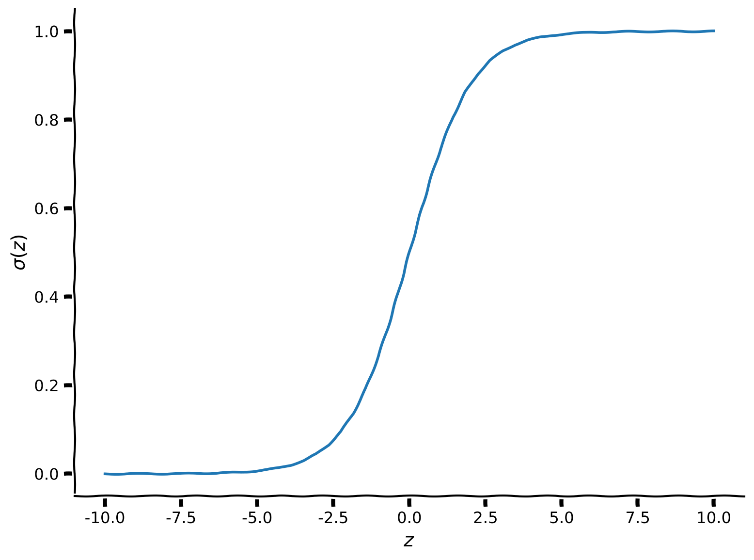
Here \(\sigma(\cdot)\) is a “squashing” function called the sigmoid function or logistic function. Its output is in the range \(0 \leq y \leq 1\). It looks like this:

(191)#\[\begin{equation} \sigma(z) = \frac{1}{1 + \textrm{exp}(-z)} \end{equation}\]

Recall that \(z = \theta^\top x\). The parameters decide whether \(\theta^\top x\) will be very negative, in which case \(\sigma(\theta^\top x)\approx 0\), or very positive, meaning \(\sigma(\theta^\top x)\approx 1\).

Coding Exercise 1.1: Implement the sigmoid function#

def sigmoid(z):
  """Return the logistic transform of z."""
  ##############################################################################
  # TODO for students: Fill in the missing code (...) and remove the error
  raise NotImplementedError("Student exercise: implement the sigmoid function")
  ##############################################################################

  sigmoid = ...

  return sigmoid


# Visualize
plot_function(sigmoid, "\sigma", "z", (-10, 10))

Click for solution

Example output:

Submit your feedback#

Section 1.2: Using scikit-learn#

Estimated timing to here from start of tutorial: 13 min

Unlike the previous notebook, we’re not going to write the code that implements all of the Logistic Regression model itself. Instead, we’re going to use the implementation in scikit-learn, a very popular library for Machine Learning.

The goal of this next section is to introduce scikit-learn classifiers and understand how to apply it to real neural data.

Section 2: Decoding neural data with logistic regression#

Section 2.1: Setting up the data#

Estimated timing to here from start of tutorial: 15 min

In this notebook we’ll use the Steinmetz dataset that you have seen previously. Recall that this dataset includes recordings of neurons as mice perform a decision task.

Mice had the task of turning a wheel to indicate whether they perceived a Gabor stimulus to the left, to the right, or not at all. Neuropixel probes measured spikes across the cortex. Check out the following task schematic below from the BiorXiv preprint.

Execute to see schematic

../../../_images/ab742090d1782fbedd67b106d2856e36a24f4947815c8c6fccc8c708d1861e95.png

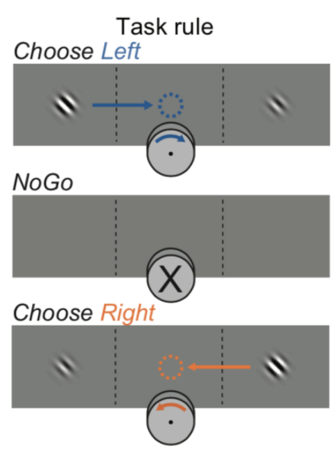
Today we’re going to decode the decision from neural data using Logistic Regression. We will only consider trials where the mouse chose “Left” or “Right” and ignore NoGo trials.

Data format#

In the hidden Data retrieval and loading cell, there is a function that loads the data:

spikes: an array of normalized spike rates with shape (n_trials, n_neurons)
choices: a vector of 0s and 1s, indicating the animal’s behavioural response, with length n_trials.

data = load_steinmetz_data()
for key, val in data.items():
  print(key, val.shape)

spikes (276, 691)
choices (276,)

As with the GLMs you’ve seen in the previous tutorial (Linear and Poisson Regression), we will need two data structures:

an X matrix with shape (n_samples, n_features)
a y vector with length n_samples.

In the previous notebook, y corresponded to the neural data, and X corresponded to something about the experiment. Here, we are going to invert those relationships. That’s what makes this a decoding model: we are going to predict behaviour (y) from the neural responses (X):

y = data["choices"]
X = data["spikes"]

Section 2.2: Fitting the model#

Estimated timing to here from start of tutorial: 25 min

Using a Logistic Regression model within scikit-learn is very simple.

# Define the model
log_reg = LogisticRegression(penalty=None)

# Fit it to data
log_reg.fit(X, y)

LogisticRegression(penalty=None)

In a Jupyter environment, please rerun this cell to show the HTML representation or trust the notebook.
On GitHub, the HTML representation is unable to render, please try loading this page with nbviewer.org.

There’s two steps here:

We initialized the model with a hyperparameter, telling it what penalty to use (we’ll focus on this in the second part of the notebook)
We fit the model by passing it the X and y objects.

Section 2.3: Classifying the training data#

Estimated timing to here from start of tutorial: 27 min

Fitting the model performs maximum likelihood optimization, learning a set of feature weights. We can use those learned weights to classify new data, or predict the labels for each sample:

y_pred = log_reg.predict(X)

Section 2.4: Evaluating the model#

Estimated timing to here from start of tutorial: 30 min

Now, we need to evaluate the predictions of the model. We will use an accuracy score for this purpose. The accuracy of a classifier is determined by the proportion of correct trials, where the predicted label matches the true label, out of the total number of trials.

Coding Exercise 2.4: Classifier accuracy#

For the first exercise, implement a function to evaluate a classifier using the accuracy score. Use it to get the accuracy of the classifier on the training data.

def compute_accuracy(X, y, model):
  """Compute accuracy of classifier predictions.

  Args:
    X (2D array): Data matrix
    y (1D array): Label vector
    model (sklearn estimator): Classifier with trained weights.

  Returns:
    accuracy (float): Proportion of correct predictions.
  """
  #############################################################################
  # TODO Complete the function, then remove the next line to test it
  raise NotImplementedError("Implement the compute_accuracy function")
  #############################################################################

  y_pred = model.predict(X)

  accuracy = ...

  return accuracy


# Compute train accuracy
train_accuracy = compute_accuracy(X, y, log_reg)
print(f"Accuracy on the training data: {train_accuracy:.2%}")

You should see

Accuracy on the training data: 100.00%

Click for solution

Submit your feedback#

Section 2.5: Cross-validating the classifier#

Estimated timing to here from start of tutorial: 40 min

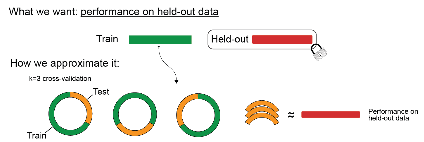
Classification accuracy on the training data is 100%! That might sound impressive, but you should recall from yesterday the concept of overfitting: the classifier may have learned something idiosyncratic about the training data. If that’s the case, it won’t have really learned the underlying data->decision function, and thus won’t generalize well to new data.

To check this, we can evaluate the cross-validated accuracy.

Execute to see schematic

../../../_images/7fe784607aaa1c49214839affe7748bad2999e818152df53f65d6898fcd79496.png

Cross-validating using `scikit-learn` helper functions#

Yesterday, we asked you to write your own functions for implementing cross-validation. In practice, this won’t be necessary, because scikit-learn offers a number of helpful functions that will do this for you. For example, you can cross-validate a classifier using cross_val_score.

cross_val_score takes a sklearn model like LogisticRegression, as well as your X and y data. It then retrains your model on test/train splits of X and y, and returns the test accuracy on each of the test sets.

accuracies = cross_val_score(LogisticRegression(penalty=None), X, y, cv=8)  # k=8 cross validation

Run to plot out these k=8 accuracy scores.

../../../_images/ea8a1738b367e57749bcf1ab7b4a943798c7271080bf8071f41153608eb83414.png

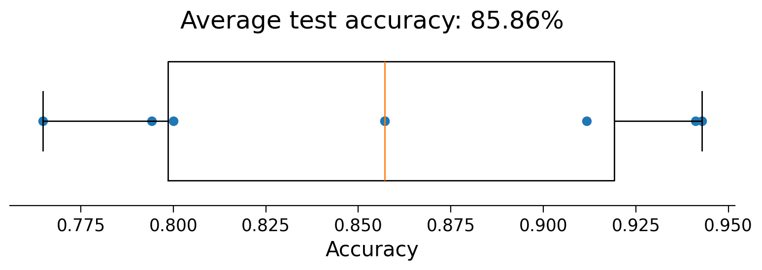
The lower cross-validated accuracy compared to the training accuracy (100%) suggests that the model is being overfit. Is this surprising? Think about the shape of the \(X\) matrix:

print(X.shape)

(276, 691)

The model has almost three times as many features as samples. This is a situation where overfitting is very likely (almost guaranteed).

Link to neuroscience: Neuro data commonly has more features than samples. Having more neurons than independent trials is one example. In fMRI data, there are commonly more measured voxels than independent trials.

Why more features than samples leads to overfitting#

In brief, the variance of model estimation increases when there are more features than samples. That is, you would get a very different model every time you get new data and run .fit(). This is very related to the bias/variance tradeoff you learned about on day 1.

Why does this happen? Here’s a tiny example to get your intuition going. Imagine trying to find a best-fit line in 2D when you only have 1 datapoint. There are simply an infinite number of lines that pass through that point. This is the situation we find ourselves in with more features than samples.

What we can do about it#

As you learned on day 1, you can decrease model variance if you don’t mind increasing its bias. Here, we will increase bias by assuming that the correct parameters are all small. In our 2D example, this is like preferring the horizontal line to all others. This is one example of regularization.

Section 3: Regularization#

Estimated timing to here from start of tutorial: 50 min

Video 2: Regularization#

Submit your feedback#

Click here for text recap of video

Regularization forces a model to learn a set solutions you a priori believe to be more correct, which reduces overfitting because it doesn’t have as much flexibility to fit idiosyncracies in the training data. This adds model bias, but it’s a good bias because you know (maybe) that parameters should be small or mostly 0.

In a GLM, a common form of regularization is to shrink the classifier weights. In a linear model, you can see its effect by plotting the weights. We’ve defined a helper function, plot_weights, that we’ll use extensively in this section.

Here is what the weights look like for a Logistic Regression model with no regularization:

log_reg = LogisticRegression(penalty=None).fit(X, y)
plot_weights({"No regularization": log_reg})

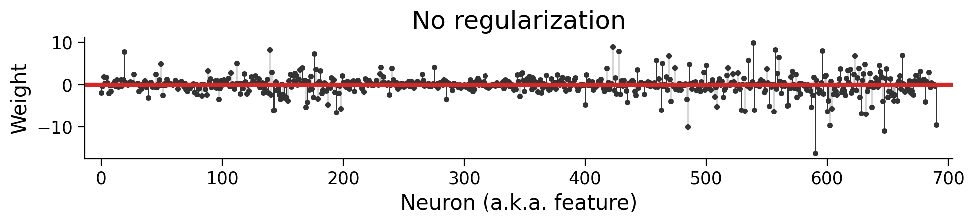
../../../_images/0085faecc620b7f9df538993af40be05e00739de49d2359830bd2e9f51579af3.png

It’s important to understand this plot. Each dot visualizes a value in our parameter vector \(\theta\). (It’s the same style of plot as the one showing \(\theta\) in the video). Since each feature is the time-averaged response of a neuron, each dot shows how the model uses each neuron to estimate a decision.

Note the scale of the y-axis. Some neurons have values of about \(20\), whereas others scale to \(-20\).

Section 3.1: \(L_2\) regularization#

Estimated timing to here from start of tutorial: 53 min

Regularization comes in different flavors. A very common one uses an \(L_2\) or “ridge” penalty. This changes the objective function to

(192)#\[\begin{equation} -\log\mathcal{L}'(\theta | X, y)= -\log\mathcal{L}(\theta | X, y) +\frac\beta2\sum_i\theta_i^2, \end{equation}\]

where \(\beta\) is a hyperparameter that sets the strength of the regularization.

You can use regularization in scikit-learn by changing the penalty, and you can set the strength of the regularization with the C hyperparameter (\(C = \frac{1}{\beta}\), so this sets the inverse regularization).

Let’s compare the unregularized classifier weights with the classifier weights when we use the default C = 1:

log_reg_l2 = LogisticRegression(penalty="l2", C=1).fit(X, y)

# now show the two models
models = {
  "No regularization": log_reg,
  "$L_2$ (C = 1)": log_reg_l2,
}
plot_weights(models)

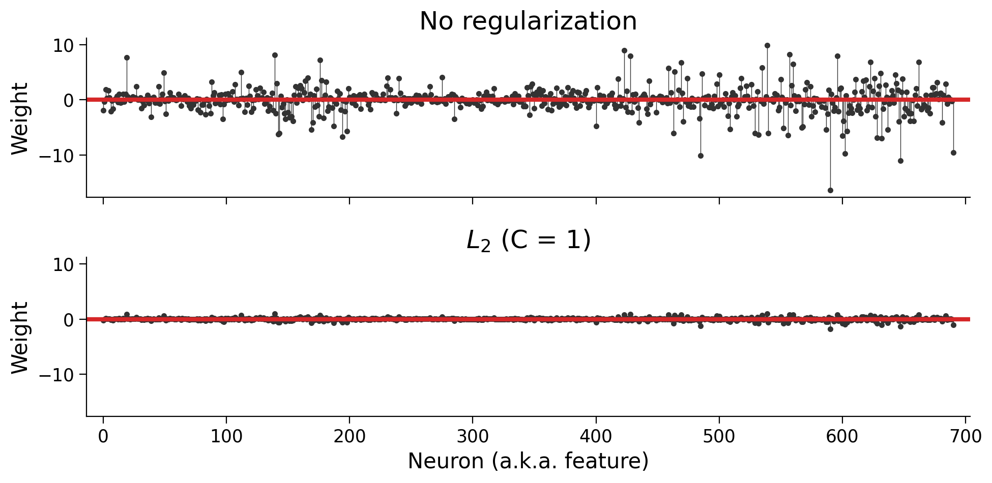
../../../_images/55be790fac18ba4e18ccd02e55af64ee2f36e83c58223ac6c504032bfee4c31b.png

Using the same scale for the two y axes, it’s almost impossible to see the \(L_2\) weights. Let’s allow the y axis scales to adjust to each set of weights:

plot_weights(models, sharey=False)

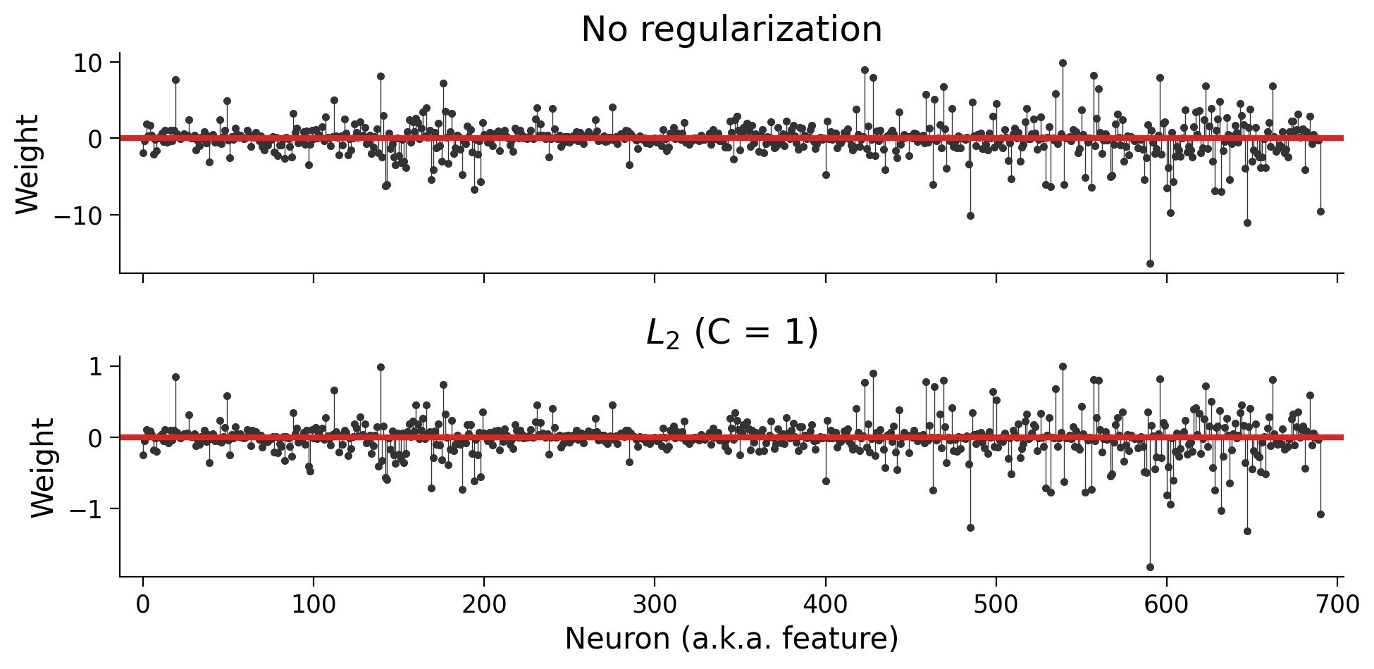
../../../_images/1e6dafb8ad1623c7c508b243404b8c214714ef2bcc21429a57276e3c7cbf1ce3.png

Now you can see that the weights have the same basic pattern, but the regularized weights are an order-of-magnitude smaller.

Interactive Demo 3.1: The effect of varying C on parameter size#

We can use this same approach to see how the weights depend on the strength of the regularization:

Execute this cell to enable the widget!

Recall from above that \(C=\frac1\beta\) so larger \(C\) is less regularization. The top panel corresponds to \(C \rightarrow \infty\).

Section 3.2: \(L_1\) regularization#

Estimated timing to here from start of tutorial: 1 hr, 3 min

\(L_2\) is not the only option for regularization. There is also the \(L_1\), or “Lasso” penalty. This changes the objective function to

(193)#\[\begin{equation} -\log\mathcal{L}'(\theta | X, y) = -\log\mathcal{L}(\theta | X, y) +\frac\beta2\sum_i|\theta_i| \end{equation}\]

In practice, using the summed absolute values of the weights causes sparsity: instead of just getting smaller, some of the weights will get forced to \(0\):

log_reg_l1 = LogisticRegression(penalty="l1", C=1, solver="saga", max_iter=5000)
log_reg_l1.fit(X, y)
models = {
  "$L_2$ (C = 1)": log_reg_l2,
  "$L_1$ (C = 1)": log_reg_l1,
}
plot_weights(models)

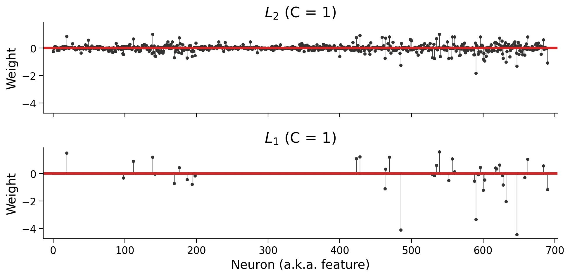
../../../_images/43aa79b6b9f4da0d53c7cf7a4045549bf31261ef6fc9a8d579ce8a7254b21557.png

Note: You’ll notice that we added two additional parameters: solver="saga" and max_iter=5000. The LogisticRegression class can use several different optimization algorithms (“solvers”), and not all of them support the \(L_1\) penalty. At a certain point, the solver will give up if it hasn’t found a minimum value. The max_iter parameter tells it to make more attempts; otherwise, we’d see an ugly warning about “convergence”.

Section 3.3: The key difference between \(L_1\) and \(L_2\) regularization: sparsity#

Estimated timing to here from start of tutorial: 1 hr, 10 min

When should you use \(L_1\) vs. \(L_2\) regularization? Both penalties shrink parameters, and both will help reduce overfitting. However, the models they lead to are different.

In particular, the \(L_1\) penalty encourages sparse solutions in which most parameters are 0. Let’s unpack the notion of sparsity.

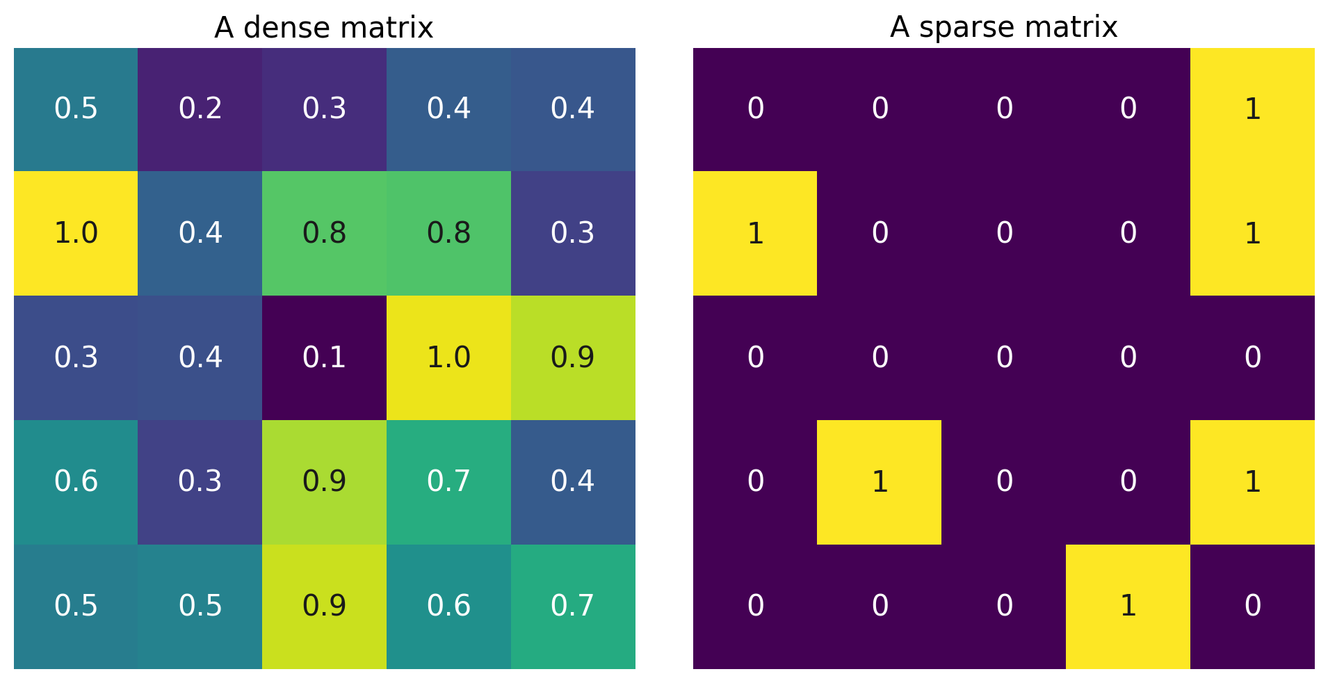
A “dense” vector has mostly nonzero elements: \(\begin{bmatrix} 0.1 \\ -0.6\\-9.1\\0.07 \end{bmatrix}\). A “sparse” vector has mostly zero elements: \(\begin{bmatrix} 0 \\ -0.7\\ 0\\0 \end{bmatrix}\).

The same is true of matrices:

Execute to plot a dense and a sparse matrix

../../../_images/41d13444eb5c679317b064e750ff330576801ba77463a68c6bca77962941ddc0.png

Coding Exercise 3.3: The effect of \(L_1\) regularization on parameter sparsity#

Please complete the following function to fit a regularized LogisticRegression model and return the number of coefficients in the parameter vector that are equal to 0.

Don’t forget to check out the scikit-learn documentation.

def count_non_zero_coefs(X, y, C_values):
  """Fit models with different L1 penalty values and count non-zero coefficients.

  Args:
    X (2D array): Data matrix
    y (1D array): Label vector
    C_values (1D array): List of hyperparameter values

  Returns:
    non_zero_coefs (list): number of coefficients in each model that are nonzero

  """
  #############################################################################
  # TODO Complete the function and remove the error
  raise NotImplementedError("Implement the count_non_zero_coefs function")
  #############################################################################

  non_zero_coefs = []
  for C in C_values:

    # Initialize and fit the model
    # (Hint, you may need to set max_iter)
    model = ...
    ...

    # Get the coefs of the fit model (in sklearn, we can do this using model.coef_)
    coefs = ...

    # Count the number of non-zero elements in coefs
    non_zero = ...
    non_zero_coefs.append(non_zero)

  return non_zero_coefs


# Use log-spaced values for C
C_values = np.logspace(-4, 4, 5)

# Count non zero coefficients
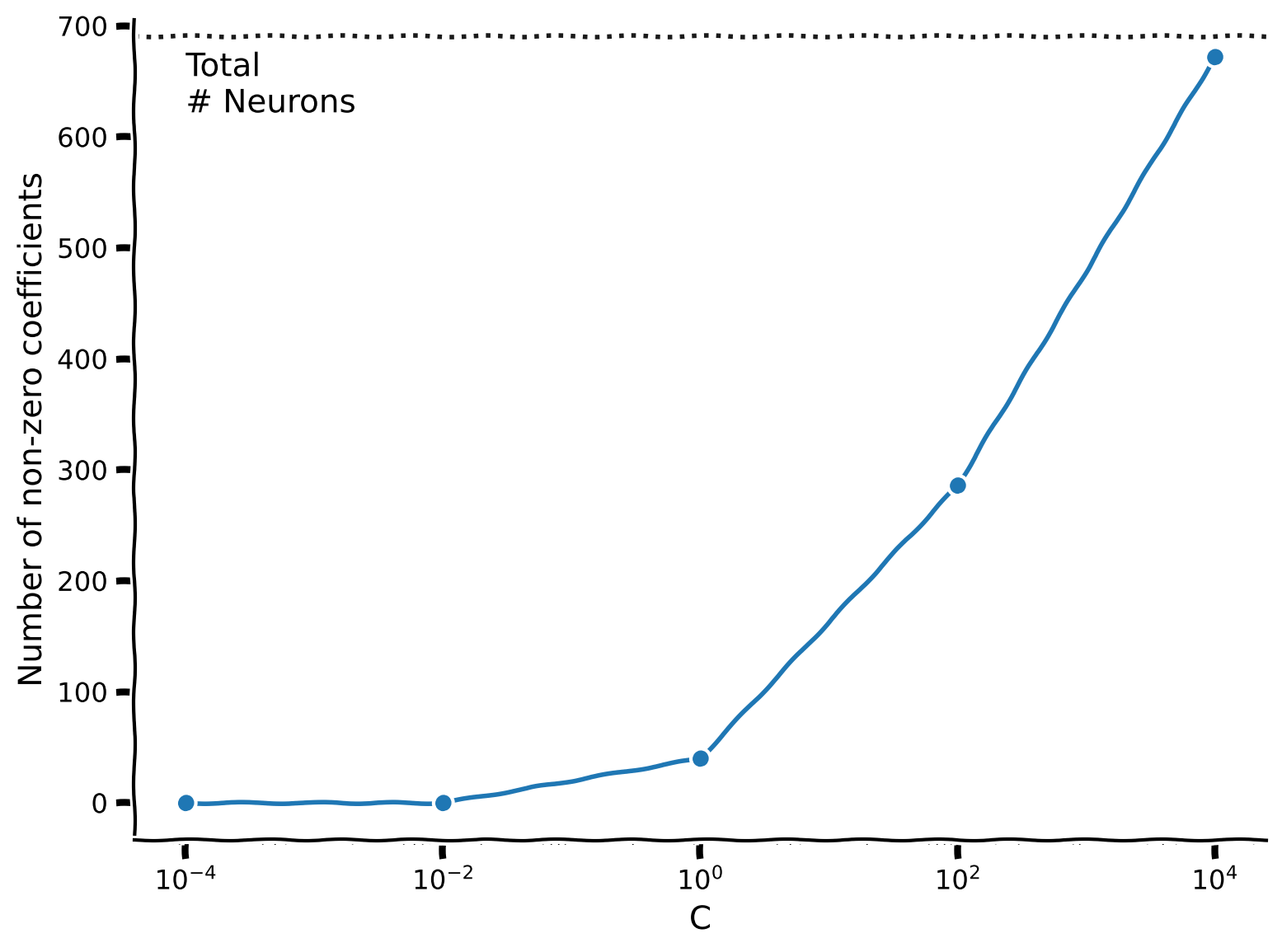
non_zero_l1 = count_non_zero_coefs(X, y, C_values)

# Visualize
plot_non_zero_coefs(C_values, non_zero_l1, n_voxels=X.shape[1])

Click for solution

Example output:

Submit your feedback#

Smaller \(C\) (bigger \(\beta\)) leads to sparser solutions.

Link to neuroscience: When is it OK to assume that the parameter vector is sparse? Whenever it is true that most features don’t affect the outcome. One use-case might be decoding low-level visual features from whole-brain fMRI: we may expect only voxels in V1 and thalamus should be used in the prediction.

WARNING: be careful when interpreting \(\theta\). Never interpret the nonzero coefficients as evidence that only those voxels/neurons/features carry information about the outcome. This is a product of our regularization scheme, and thus our prior assumption that the solution is sparse. Other regularization types or models may find very distributed relationships across the brain. Never use a model as evidence for a phenomena when that phenomena is encoded in the assumptions of the model.

Section 3.4: Choosing the regularization penalty#

Estimated timing to here from start of tutorial: 1 hr, 25 min

In the examples above, we just picked arbitrary numbers for the strength of regularization. How do you know what value of the hyperparameter to use?

The answer is the same as when you want to know whether you have learned good parameter values: use cross-validation. The best hyperparameter will be the one that allows the model to generalize best to unseen data.

Coding Exercise 3.4: Model selection#

In the final exercise, we will use cross-validation to evaluate a set of models, each with a different \(L_2\) penalty. Your model_selection function should have a for-loop that gets the mean cross-validated accuracy for each penalty value (use the cross_val_score function that we introduced above, with 8 folds).

def model_selection(X, y, C_values):
  """Compute CV accuracy for each C value.

  Args:
    X (2D array): Data matrix
    y (1D array): Label vector
    C_values (1D array): Array of hyperparameter values

  Returns:
    accuracies (1D array): CV accuracy with each value of C

  """
  #############################################################################
  # TODO Complete the function and remove the error
  raise NotImplementedError("Implement the model_selection function")
  #############################################################################

  accuracies = []
  for C in C_values:

    # Initialize and fit the model
    # (Hint, you may need to set max_iter)
    model = ...

    # Get the accuracy for each test split using cross-validation
    accs = ...

    # Store the average test accuracy for this value of C
    accuracies.append(...)

  return accuracies


# Use log-spaced values for C
C_values = np.logspace(-4, 4, 9)

# Compute accuracies
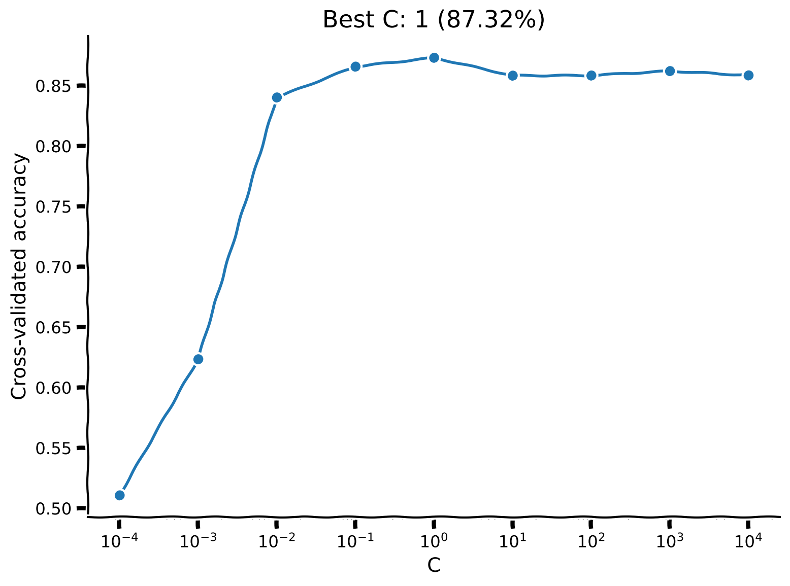
accuracies = model_selection(X, y, C_values)

# Visualize
plot_model_selection(C_values, accuracies)

Click for solution

Example output:

Submit your feedback#

This plot suggests that the right value of \(C\) does matter — up to a point. Remember that C is the inverse regularization. The plot shows that models where the regularization was too strong (small C values) performed very poorly. For \(C > 10^{-2}\), the differences are marginal, but the best performance was obtained with an intermediate value (\(C \approx 10^1\)).

Summary#

Estimated timing of tutorial: 1 hour, 35 minutes

In this notebook, we learned about Logistic Regression, a fundamental algorithm for classification. We applied the algorithm to a neural decoding problem: we tried to predict an animal’s behavioural choice from its neural activity. We saw again how important it is to use cross-validation to evaluate complex models that are at risk for overfitting, and we learned how regularization can be used to fit models that generalize better. Finally, we learned about some of the different options for regularization, and we saw how cross-validation can be useful for model selection.

Notation#

(194)#\[\begin{align} x &\quad \text{input}\\ y &\quad \text{measurement, response}\\ \theta &\quad \text{parameter}\\ \sigma(z) &\quad \text{logistic function}\\ C &\quad \text{inverse regularization strength parameter}\\ \beta &\quad \text{regularization strength parameter}\\ \hat{y} &\quad \text{estimated output}\\ \mathcal{L}(\theta| y_i, x_i) &\quad \text{likelihood of that parameter } \theta \text{ producing response } y_i \text{ from input } x_i\\ L_1 &\quad \text{Lasso regularization}\\ L_2 &\quad \text{ridge regularization}\\ \end{align}\]

Bonus#

Bonus Section 1: The Logistic Regression model in full#

The fundamental input/output equation of logistic regression is:

(195)#\[\begin{equation} p(y_i = 1 |x_i, \theta) = \sigma(\theta^\top x_i) \end{equation}\]

The logistic link function

You’ve seen \(\theta^T x_i\) before, but the \(\sigma\) is new. It’s the sigmoidal or logistic link function that “squashes” \(\theta^\top x_i\) to keep it between \(0\) and \(1\):

(196)#\[\begin{equation} \sigma(z) = \frac{1}{1 + \textrm{exp}(-z)} \end{equation}\]

The Bernoulli likelihood

You might have noticed that the output of the sigmoid, \(\hat{y}\) is not a binary value (0 or 1), even though the true data \(y\) is! Instead, we interpret the value of \(\hat{y}\) as the probability that y = 1:

(197)#\[\begin{equation} \hat{y_i} \equiv p(y_i=1|x_i,\theta) = \frac{1}{{1 + \textrm{exp}(-\theta^\top x_i)}} \end{equation}\]

To get the likelihood of the parameters, we need to define the probability of seeing \(y\) given \(\hat{y}\). In logistic regression, we do this using the Bernoulli distribution:

(198)#\[\begin{equation} P(y_i\ |\ \hat{y}_i) = \hat{y}_i^{y_i}(1 - \hat{y}_i)^{(1 - y_i)} \end{equation}\]

So plugging in the regression model:

(199)#\[\begin{equation} P(y_i\ |\ \theta, x_i) = \sigma(\theta^\top x_i)^{y_i}\left(1 - \sigma(\theta^\top x_i)\right)^{(1 - y_i)}. \end{equation}\]

This expression effectively measures how good our parameters \(\theta\) are. We can also write it as the likelihood of the parameters given the data:

(200)#\[\begin{equation} \mathcal{L}(\theta\ |\ y_i, x_i) = P(y_i\ |\ \theta, x_i), \end{equation}\]

and then use this as a target of optimization, considering all of the trials independently:

(201)#\[\begin{equation} \log\mathcal{L}(\theta | X, y) = \sum_{i=1}^Ny_i\log\left(\sigma(\theta^\top x_i)\right)\ +\ (1-y_i)\log\left(1 - \sigma(\theta^\top x_i)\right). \end{equation}\]

Bonus Section 2: More detail about model selection#

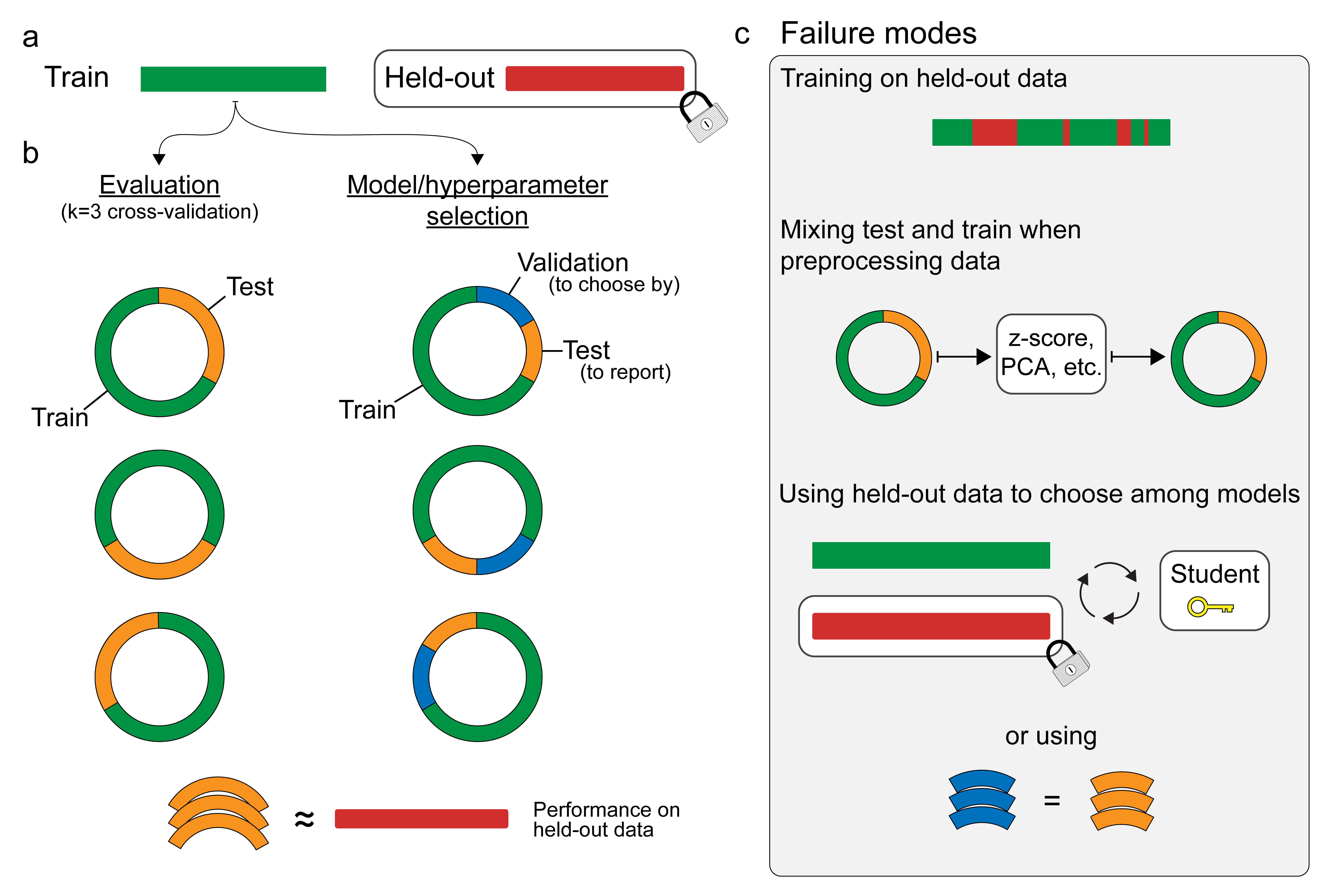
In the final exercise, we used all of the data to choose the hyperparameters. That means we don’t have any fresh data left over to evaluate the performance of the selected model. In practice, you would want to have two nested layers of cross-validation, where the final evaluation is performed on data that played no role in selecting or training the model.

Indeed, the proper method for splitting your data to choose hyperparameters can get confusing. Here’s a guide that the authors of this notebook developed while writing a tutorial on using machine learning for neural decoding arxiv:1708.00909.

Execute to see schematic

../../../_images/6126b35c314b1f3f889a8302cd3643cd85881a3ea1ba4fed9cdd48faf624081e.png

Tutorial 2: Classifiers and regularizers

Contents

Tutorial 2: Classifiers and regularizers#

Tutorial Objectives#

Setup#

Install and import feedback gadget#

Figure settings#

Plotting Functions#

Data retrieval and loading#

Section 1: Logistic regression#

Video 1: Logistic regression#

Submit your feedback#

Section 1.1: The logistic regression model#

Coding Exercise 1.1: Implement the sigmoid function#

Submit your feedback#

Section 1.2: Using scikit-learn#

Section 2: Decoding neural data with logistic regression#

Section 2.1: Setting up the data#

Data format#

Section 2.2: Fitting the model#

Section 2.3: Classifying the training data#

Section 2.4: Evaluating the model#

Coding Exercise 2.4: Classifier accuracy#

Submit your feedback#

Section 2.5: Cross-validating the classifier#

Cross-validating using scikit-learn helper functions#

Why more features than samples leads to overfitting#

What we can do about it#

Section 3: Regularization#

Video 2: Regularization#

Submit your feedback#

Section 3.1: \(L_2\) regularization#

Interactive Demo 3.1: The effect of varying C on parameter size#

Section 3.2: \(L_1\) regularization#

Section 3.3: The key difference between \(L_1\) and \(L_2\) regularization: sparsity#

Coding Exercise 3.3: The effect of \(L_1\) regularization on parameter sparsity#

Submit your feedback#

Section 3.4: Choosing the regularization penalty#

Coding Exercise 3.4: Model selection#

Submit your feedback#

Summary#

Notation#

Bonus#

Bonus Section 1: The Logistic Regression model in full#

Bonus Section 2: More detail about model selection#

Cross-validating using `scikit-learn` helper functions#