Tutorial 3: Building and Evaluating Normative Encoding Models

Tutorial 3: Building and Evaluating Normative Encoding Models#

Week 1, Day 5: Deep Learning

By Neuromatch Academy

Content creators: Jorge A. Menendez, Yalda Mohsenzadeh, Carsen Stringer

Content reviewers: Roozbeh Farhoodi, Madineh Sarvestani, Kshitij Dwivedi, Spiros Chavlis, Ella Batty, Michael Waskom

Production editors: Spiros Chavlis

Tutorial Objectives#

Estimated timing of tutorial: 1 hour, 10 minutes

In this tutorial, we’ll be using deep learning to build an encoding model of the visual system, and then compare its internal representations to those observed in neural data.

Its parameters won’t be directly optimized to fit the neural data. Instead, we will optimize its parameters to solve a particular visual task that we know the brain can solve. We therefore refer to it as a “normative” encoding model, since it is optimized for a specific behavioral task. It is the optimal model to solve the problem (optimal for the specified architecture). See Section 3 of the bonus tutorial to fit a convolutional neural network directly to neural data (an alternative approach for investigating encoding with deep neural networks).

To then evaluate whether this normative encoding model is actually a good model of the brain, we’ll analyze its internal representations and compare them to the representations observed in the mouse primary visual cortex. Since we understand exactly what the encoding model’s representations are optimized to do, any similarities will hopefully shed light on why the representations in the brain look the way they do.

More concretely, our goal will be learn how to:

Visualize and analyze the internal representations of a deep network
Quantify the similarity between distributed representations in a model and neural representations observed in recordings, using Representational Similarity Analysis (RSA)

Setup#

Install and import feedback gadget#

# Imports
import numpy as np
from scipy.stats import zscore
import matplotlib as mpl
from matplotlib import pyplot as plt

import torch
from torch import nn, optim
from sklearn.decomposition import PCA
from sklearn.manifold import TSNE

Figure Settings#

Plotting Functions#

Show code cell source Hide code cell source

# @title Plotting Functions

def show_stimulus(img, ax=None, show=False):
  """Visualize a stimulus"""
  if ax is None:
    ax = plt.gca()
  ax.imshow(img, cmap=mpl.cm.binary)
  ax.set_aspect('auto')
  ax.set_xticks([])
  ax.set_yticks([])
  ax.spines['left'].set_visible(False)
  ax.spines['bottom'].set_visible(False)
  if show:
    plt.show()


def plot_corr_matrix(rdm, ax=None, show=False):
  """Plot dissimilarity matrix

  Args:
    rdm (numpy array): n_stimuli x n_stimuli representational dissimilarity
      matrix
    ax (matplotlib axes): axes onto which to plot

  Returns:
    nothing

  """
  if ax is None:
    ax = plt.gca()
  image = ax.imshow(rdm, vmin=0.0, vmax=2.0)
  ax.set_xticks([])
  ax.set_yticks([])
  cbar = plt.colorbar(image, ax=ax, label='dissimilarity')
  if show:
    plt.show()


def plot_multiple_rdm(rdm_dict):
  """Draw multiple subplots for each RDM in rdm_dict."""
  fig, axs = plt.subplots(1, len(rdm_dict),
                          figsize=(4 * len(resp_dict), 3.5))

  # Compute RDM's for each set of responses and plot
  for i, (label, rdm) in enumerate(rdm_dict.items()):

    image = plot_corr_matrix(rdm, axs[i])
    axs[i].set_title(label)
  plt.show()


def plot_rdm_rdm_correlations(rdm_sim):
  """Draw a bar plot showing between-RDM correlations."""
  f, ax = plt.subplots()
  ax.bar(rdm_sim.keys(), rdm_sim.values())
  ax.set_xlabel('Deep network model layer')
  ax.set_ylabel('Correlation of model layer RDM\nwith mouse V1 RDM')
  plt.show()


def plot_rdm_rows(ori_list, rdm_dict, rdm_oris):
  """Plot the dissimilarity of response to each stimulus with response to one
  specific stimulus

  Args:
    ori_list (list of float): plot dissimilarity with response to stimulus with
      orientations closest to each value in this list
    rdm_dict (dict): RDM's from which to extract dissimilarities
    rdm_oris (np.ndarray): orientations corresponding to each row/column of RDMs
    in rdm_dict

  """
  n_col = len(ori_list)
  f, axs = plt.subplots(1, n_col, figsize=(4 * n_col, 4), sharey=True)

  # Get index of orientation closest to ori_plot
  for ax, ori_plot in zip(axs, ori_list):
    iori = np.argmin(np.abs(rdm_oris - ori_plot))

    # Plot dissimilarity curves in each RDM
    for label, rdm in rdm_dict.items():
      ax.plot(rdm_oris, rdm[iori, :], label=label)

    # Draw vertical line at stimulus we are plotting dissimilarity w.r.t.
    ax.axvline(rdm_oris[iori], color=".7", zorder=-1)

    # Label axes
    ax.set_title(f'Dissimilarity with response\nto {ori_plot: .0f}$^o$ stimulus')
    ax.set_xlabel('Stimulus orientation ($^o$)')

  axs[0].set_ylabel('Dissimilarity')
  axs[-1].legend(loc="upper left", bbox_to_anchor=(1, 1))
  plt.tight_layout()
  plt.show()

Helper Functions#

Show code cell source Hide code cell source

# @title Helper Functions

def load_data(data_name, bin_width=1):
  """Load mouse V1 data from Stringer et al. (2019)

  Data from study reported in this preprint:
  https://www.biorxiv.org/content/10.1101/679324v2.abstract

  These data comprise time-averaged responses of ~20,000 neurons
  to ~4,000 stimulus gratings of different orientations, recorded
  through Calcium imaginge. The responses have been normalized by
  spontanous levels of activity and then z-scored over stimuli, so
  expect negative numbers. They have also been binned and averaged
  to each degree of orientation.

  This function returns the relevant data (neural responses and
  stimulus orientations) in a torch.Tensor of data type torch.float32
  in order to match the default data type for nn.Parameters in
  Google Colab.

  This function will actually average responses to stimuli with orientations
  falling within bins specified by the bin_width argument. This helps
  produce individual neural "responses" with smoother and more
  interpretable tuning curves.

  Args:
    bin_width (float): size of stimulus bins over which to average neural
      responses

  Returns:
    resp (torch.Tensor): n_stimuli x n_neurons matrix of neural responses,
        each row contains the responses of each neuron to a given stimulus.
        As mentioned above, neural "response" is actually an average over
        responses to stimuli with similar angles falling within specified bins.
    stimuli: (torch.Tensor): n_stimuli x 1 column vector with orientation
        of each stimulus, in degrees. This is actually the mean orientation
        of all stimuli in each bin.

  """
  with np.load(data_name) as dobj:
    data = dict(**dobj)
  resp = data['resp']
  stimuli = data['stimuli']

  if bin_width > 1:
    # Bin neural responses and stimuli
    bins = np.digitize(stimuli, np.arange(0, 360 + bin_width, bin_width))
    stimuli_binned = np.array([stimuli[bins == i].mean() for i in np.unique(bins)])
    resp_binned = np.array([resp[bins == i, :].mean(0) for i in np.unique(bins)])
  else:
    resp_binned = resp
    stimuli_binned = stimuli

  # only use stimuli <= 180
  resp_binned = resp_binned[stimuli_binned <= 180]
  stimuli_binned = stimuli_binned[stimuli_binned <= 180]

  stimuli_binned -= 90  # 0 means vertical, -ve means tilted left, +ve means tilted right

  # Return as torch.Tensor
  resp_tensor = torch.tensor(resp_binned, dtype=torch.float32)
  stimuli_tensor = torch.tensor(stimuli_binned, dtype=torch.float32).unsqueeze(1)  # add singleton dimension to make a column vector

  return resp_tensor, stimuli_tensor


def grating(angle, sf=1 / 28, res=0.1, patch=False):
  """Generate oriented grating stimulus

  Args:
    angle (float): orientation of grating (angle from vertical), in degrees
    sf (float): controls spatial frequency of the grating
    res (float): resolution of image. Smaller values will make the image
      smaller in terms of pixels. res=1.0 corresponds to 640 x 480 pixels.
    patch (boolean): set to True to make the grating a localized
      patch on the left side of the image. If False, then the
      grating occupies the full image.

  Returns:
    torch.Tensor: (res * 480) x (res * 640) pixel oriented grating image

  """

  angle = np.deg2rad(angle)  # transform to radians

  wpix, hpix = 640, 480  # width and height of image in pixels for res=1.0

  xx, yy = np.meshgrid(sf * np.arange(0, wpix * res) / res, sf * np.arange(0, hpix * res) / res)

  if patch:
    gratings = np.cos(xx * np.cos(angle + .1) + yy * np.sin(angle + .1))  # phase shift to make it better fit within patch
    gratings[gratings < 0] = 0
    gratings[gratings > 0] = 1
    xcent = gratings.shape[1] * .75
    ycent = gratings.shape[0] / 2
    xxc, yyc = np.meshgrid(np.arange(0, gratings.shape[1]), np.arange(0, gratings.shape[0]))
    icirc = ((xxc - xcent) ** 2 + (yyc - ycent) ** 2) ** 0.5 < wpix / 3 / 2 * res
    gratings[~icirc] = 0.5

  else:
    gratings = np.cos(xx * np.cos(angle) + yy * np.sin(angle))
    gratings[gratings < 0] = 0
    gratings[gratings > 0] = 1

  # Return torch tensor
  return torch.tensor(gratings, dtype=torch.float32)


def filters(out_channels=6, K=7):
  """ make example filters, some center-surround and gabors
  Returns:
      filters: out_channels x K x K
  """
  grid = np.linspace(-K/2, K/2, K).astype(np.float32)
  xx,yy = np.meshgrid(grid, grid, indexing='ij')

  # create center-surround filters
  sigma = 1.1
  gaussian = np.exp(-(xx**2 + yy**2)**0.5/(2*sigma**2))
  wide_gaussian = np.exp(-(xx**2 + yy**2)**0.5/(2*(sigma*2)**2))
  center_surround = gaussian - 0.5 * wide_gaussian

  # create gabor filters
  thetas = np.linspace(0, 180, out_channels-2+1)[:-1] * np.pi/180
  gabors = np.zeros((len(thetas), K, K), np.float32)
  lam = 10
  phi = np.pi/2
  gaussian = np.exp(-(xx**2 + yy**2)**0.5/(2*(sigma*0.4)**2))
  for i,theta in enumerate(thetas):
    x = xx*np.cos(theta) + yy*np.sin(theta)
    gabors[i] = gaussian * np.cos(2*np.pi*x/lam + phi)

  filters = np.concatenate((center_surround[np.newaxis,:,:],
                            -1*center_surround[np.newaxis,:,:],
                            gabors),
                           axis=0)
  filters /= np.abs(filters).max(axis=(1,2))[:,np.newaxis,np.newaxis]
  # convert to torch
  filters = torch.from_numpy(filters)
  # add channel axis
  filters = filters.unsqueeze(1)

  return filters


class CNN(nn.Module):
  """Deep convolutional network with one convolutional + pooling layer followed
  by one fully connected layer

  Args:
    h_in (int): height of input image, in pixels (i.e. number of rows)
    w_in (int): width of input image, in pixels (i.e. number of columns)

  Attributes:
    conv (nn.Conv2d): filter weights of convolutional layer
    pool (nn.MaxPool2d): max pooling layer
    dims (tuple of ints): dimensions of output from pool layer
    fc (nn.Linear): weights and biases of fully connected layer
    out (nn.Linear): weights and biases of output layer

  """

  def __init__(self, h_in, w_in):
    super().__init__()
    C_in = 1  # input stimuli have only 1 input channel
    C_out = 6  # number of output channels (i.e. of convolutional kernels to convolve the input with)
    K = 7  # size of each convolutional kernel
    Kpool = 8  # size of patches over which to pool
    self.conv = nn.Conv2d(C_in, C_out, kernel_size=K, padding=K//2)  # add padding to ensure that each channel has same dimensionality as input
    self.pool = nn.MaxPool2d(Kpool)
    self.dims = (C_out, h_in // Kpool, w_in // Kpool)  # dimensions of pool layer output
    self.fc = nn.Linear(np.prod(self.dims), 10)  # flattened pool output --> 10D representation
    self.out = nn.Linear(10, 1)  # 10D representation --> scalar
    self.conv.weight = nn.Parameter(filters(C_out, K))
    self.conv.bias = nn.Parameter(torch.zeros((C_out,), dtype=torch.float32))

  def forward(self, x):
    """Classify grating stimulus as tilted right or left

    Args:
      x (torch.Tensor): p x 48 x 64 tensor with pixel grayscale values for
          each of p stimulus images.

    Returns:
      torch.Tensor: p x 1 tensor with network outputs for each input provided
          in x. Each output should be interpreted as the probability of the
          corresponding stimulus being tilted right.

    """
    x = x.unsqueeze(1)  # p x 1 x 48 x 64, add a singleton dimension for the single stimulus channel
    x = torch.relu(self.conv(x))  # output of convolutional layer
    x = self.pool(x)  # output of pooling layer
    x = x.view(-1, np.prod(self.dims))  # flatten pooling layer outputs into a vector
    x = torch.relu(self.fc(x))  # output of fully connected layer
    x = torch.sigmoid(self.out(x))  # network output
    return x


def train(net, train_data, train_labels,
          n_epochs=25, learning_rate=0.0005,
          batch_size=100, momentum=.99):
  """Run stochastic gradient descent on binary cross-entropy loss for a given
  deep network (cf. appendix for details)

  Args:
    net (nn.Module): deep network whose parameters to optimize with SGD
    train_data (torch.Tensor): n_train x h x w tensor with stimulus gratings
    train_labels (torch.Tensor): n_train x 1 tensor with true tilt of each
      stimulus grating in train_data, i.e. 1. for right, 0. for left
    n_epochs (int): number of times to run SGD through whole training data set
    batch_size (int): number of training data samples in each mini-batch
    learning_rate (float): learning rate to use for SGD updates
    momentum (float): momentum parameter for SGD updates

  """

  # Initialize binary cross-entropy loss function
  loss_fn = nn.BCELoss()

  # Initialize SGD optimizer with momentum
  optimizer = optim.SGD(net.parameters(), lr=learning_rate, momentum=momentum)

  # Placeholder to save loss at each iteration
  track_loss = []

  # Loop over epochs
  for i in range(n_epochs):

    # Split up training data into random non-overlapping mini-batches
    ishuffle = torch.randperm(train_data.shape[0])  # random ordering of training data
    minibatch_data = torch.split(train_data[ishuffle], batch_size)  # split train_data into minibatches
    minibatch_labels = torch.split(train_labels[ishuffle], batch_size)  # split train_labels into minibatches

    # Loop over mini-batches
    for stimuli, tilt in zip(minibatch_data, minibatch_labels):

      # Evaluate loss and update network weights
      out = net(stimuli)  # predicted probability of tilt right
      loss = loss_fn(out, tilt)  # evaluate loss
      optimizer.zero_grad()  # clear gradients
      loss.backward()  # compute gradients
      optimizer.step()  # update weights

      # Keep track of loss at each iteration
      track_loss.append(loss.item())

    # Track progress
    if (i + 1) % (n_epochs // 5) == 0:
      print(f'epoch {i + 1} | loss on last mini-batch: {loss.item(): .2e}')

  print('training done!')


def get_hidden_activity(net, stimuli, layer_labels):
  """Retrieve internal representations of network

  Args:
    net (nn.Module): deep network
    stimuli (torch.Tensor): p x 48 x 64 tensor with stimuli for which to
      compute and retrieve internal representations
    layer_labels (list): list of strings with labels of each layer for which
      to return its internal representations

  Returns:
    dict: internal representations at each layer of the network, in
      numpy arrays. The keys of this dict are the strings in layer_labels.

  """

  # Placeholder
  hidden_activity = {}

  # Attach 'hooks' to each layer of the network to store hidden
  # representations in hidden_activity
  def hook(module, input, output):
    module_label = list(net._modules.keys())[np.argwhere([module == m for m in net._modules.values()])[0, 0]]
    if module_label in layer_labels:  # ignore output layer
      hidden_activity[module_label] = output.view(stimuli.shape[0], -1).detach().numpy()
  hooks = [layer.register_forward_hook(hook) for layer in net.children()]

  # Run stimuli through the network
  pred = net(stimuli)

  # Remove the hooks
  [h.remove() for h in hooks]

  return hidden_activity

Data retrieval and loading#

Section 1: Setting up deep network and neural data#

In the future sections, we will compare the activity in a deep network, specifically in a CNN, with neural activity. First, we need to understand the task we are using (Section 1.1), train our deep network (Section 1.2), and load in neural data (Section 1.3).

Video 1: Deep convolutional network for orientation discrimination#

Submit your feedback#

Section 1.1: Orientation discrimination task#

We will build our normative encoding model by optimizing its parameters to solve an orientation discrimination task.

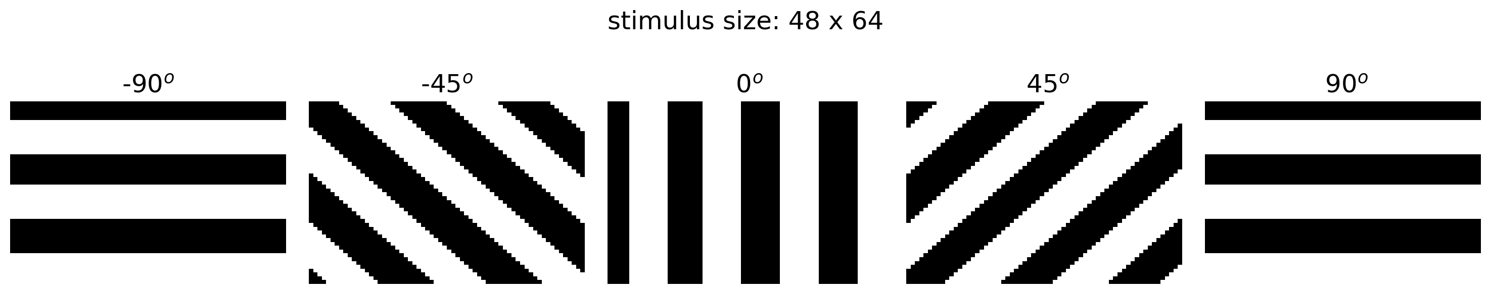
The task is to tell whether a given grating stimulus is tilted to the “right” or “left”; that is, whether its angle relative to the vertical is positive or negative, respectively. We show example stimuli below, which were constructed using the helper function grating().

Note that this is a task that we know many mammalian visual systems are capable of solving. It is therefore conceivable that the representations in a deep network model optimized for this task might resemble those in the brain. To test this hypothesis, we will compare the representations of our optimized encoding model to neural activity recorded in response to these very same stimuli, courtesy of Stringer et al 2019.

Execute this cell to plot example stimuli

../../../_images/e553f4e51a9ff168e7582876dbd1278c76b4a33d56cbf393c2c4559d5d9d464f.png

Section 1.2: A deep network model of orientation discrimination#

Estimated timing to here from start of tutorial: 10 min

Our goal is to build a model that solves the orientation discrimination task outlined above. The model should take as input a stimulus image and output the probability of that stimulus being tilted right.

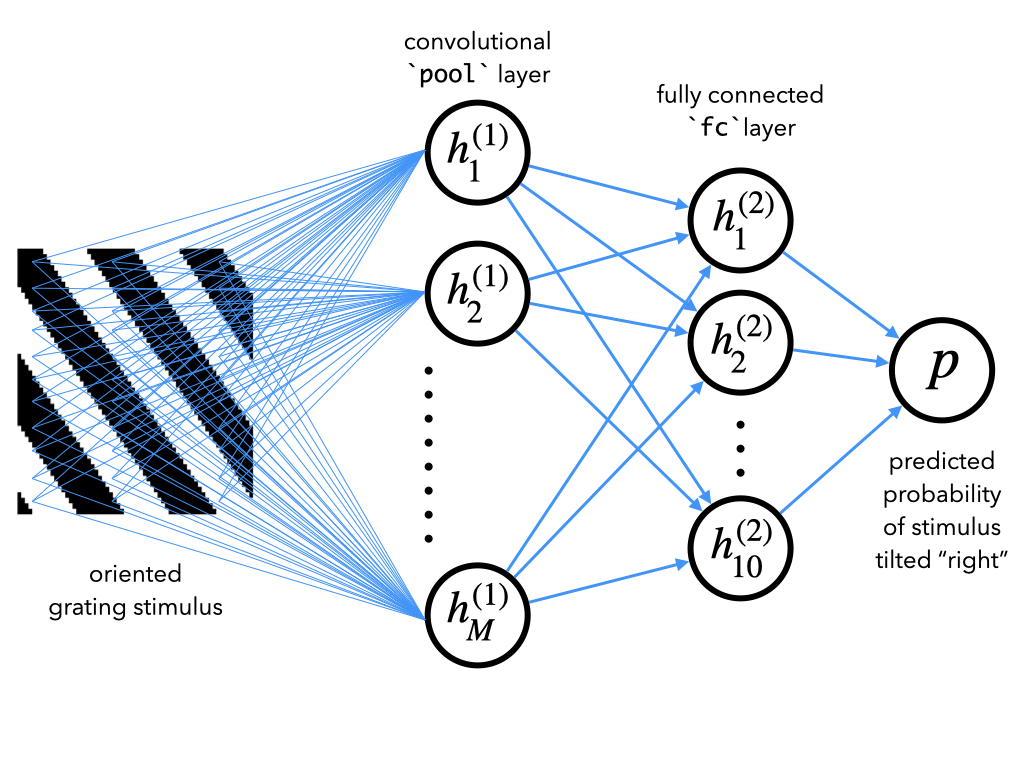
To do this, we will use a convolutional neural network (CNN), which is the type of network we saw in Tutorial 2. Here, we will use a CNN that performs two-dimensional convolutions on the raw stimulus image (which is a 2D matrix of pixels), rather than one-dimensional convolutions on a categorical 1D vector representation of the stimulus. CNNs are commonly used for image processing.

The particular CNN we will use here has two layers:

a convolutional layer, which convolves the images with a set of filters
a fully connected layer, which transforms the output of this convolution into a 10-dimensional representation

Finally, a set of output weights transforms this 10-dimensional representation into a single scalar \(p\), denoting the predicted probability of the input stimulus being tilted right.

See bonus section 1 for in-depth instructions for how to code up such a network in PyTorch. For now, however, we’ll leave these details aside and focus on training this network, called CNN, and analyzing its internal representations.

Run the next cell to train such a network to solve this task. After initializing our CNN model, it builds a dataset of oriented grating stimuli to use for training it. These are then passed into a function called train() that uses SGD to optimize the model’s parameters, taking similar arguments as the train() function we wrote in Tutorial 1.

Note that it may take ~30 seconds for the training to complete.

help(train)

Help on function train in module __main__:

train(net, train_data, train_labels, n_epochs=25, learning_rate=0.0005, batch_size=100, momentum=0.99)
    Run stochastic gradient descent on binary cross-entropy loss for a given
    deep network (cf. appendix for details)
    
    Args:
      net (nn.Module): deep network whose parameters to optimize with SGD
      train_data (torch.Tensor): n_train x h x w tensor with stimulus gratings
      train_labels (torch.Tensor): n_train x 1 tensor with true tilt of each
        stimulus grating in train_data, i.e. 1. for right, 0. for left
      n_epochs (int): number of times to run SGD through whole training data set
      batch_size (int): number of training data samples in each mini-batch
      learning_rate (float): learning rate to use for SGD updates
      momentum (float): momentum parameter for SGD updates

# Set random seeds for reproducibility
np.random.seed(12)
torch.manual_seed(12)

# Initialize CNN model
net = CNN(h, w)

# Build training set to train it on
n_train = 1000  # size of training set

# sample n_train random orientations between -90 and +90 degrees
ori = (np.random.rand(n_train) - 0.5) * 180

# build orientated grating stimuli
stimuli = torch.stack([grating(i) for i in ori])

# stimulus tilt: 1. if tilted right, 0. if tilted left, as a column vector
tilt = torch.tensor(ori > 0).type(torch.float).unsqueeze(-1)

# Train model
train(net, stimuli, tilt)

epoch 5 | loss on last mini-batch:  4.10e-01

epoch 10 | loss on last mini-batch:  5.17e-02

epoch 15 | loss on last mini-batch:  1.32e-02

epoch 20 | loss on last mini-batch:  2.27e-03

epoch 25 | loss on last mini-batch:  8.15e-05
training done!

Section 1.3: Load data#

Estimated timing to here from start of tutorial: 15 min

In the next cell, we provide code for loading in some data from Stringer et al., 2021, which contains the responses of about ~20,000 neurons in the mouse primary visual cortex to grating stimuli like those used to train our network (this is the same data used in Tutorial 1). These data are stored in two variables:

resp_v1 is a matrix where each row contains the responses of all neurons to a single stimulus.
ori is a vector with the orientations of each stimulus, in degrees. As in the above convention, negative angles denote stimuli tilted to the left and positive angles denote stimuli tilted to the right.

We will then extract our deep CNN model’s representations of these same stimuli (i.e. oriented gratings with the orientations in ori). We will run the same stimuli through our CNN model and use the helper function get_hidden_activity() to store the model’s internal representations. The output of this function is a Python dict, which contains a matrix of population responses (just like resp_v1) for each layer of the network specified by the layer_labels argument. We’ll focus on looking at the representations in

the output of the first convolutional layer, stored in the model as 'pool' (see Bonus Section 1 for the details of the CNN architecture to understand why it’s called this way)
the 10-dimensional output of the fully connected layer, stored in the model as 'fc'

# Load mouse V1 data
resp_v1, ori = load_data(fname)

# Extract model internal representations of each stimulus in the V1 data
# construct grating stimuli for each orientation presented in the V1 data
stimuli = torch.stack([grating(a.item()) for a in ori])
layer_labels = ['pool', 'fc']
resp_model = get_hidden_activity(net, stimuli, layer_labels)

# Aggregate all responses into one dict
resp_dict = {}
resp_dict['V1 data'] = resp_v1
for k, v in resp_model.items():
  label = f"model\n'{k}' layer"
  resp_dict[label] = v

Section 2: Quantitative comparisons of CNNs and neural activity#

Estimated timing to here from start of tutorial: 20 min

Let’s now analyze the internal representations of our deep CNN model of orientation discrimination and compare them to population responses in the mouse primary visual cortex.

In this section, we’ll try to quantitatively compare CNN and primary visual cortex representations. In the next section, we will visualize their representations and get some intuition for their structure.

Video 2: Quantitative comparisons of CNNs and neural activity#

Submit your feedback#

We noticed above some similarities and differences between the population responses in the mouse primary visual cortex and in different layers in our model. Let’s now try to quantify this.

To do this, we’ll use a technique called Representational Similarity Analysis. The idea is to look at the similarity structure between representations of different stimuli. We can say that a brain area and a model use a similar representational scheme if stimuli that are represented (dis)similarly in the brain are represented (dis)similarly in the model as well.

Section 2.1: Representational dissimilarity matrix (RDM)#

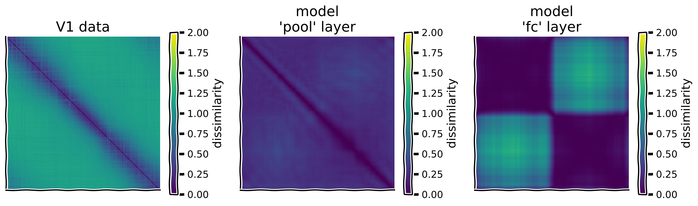
To quantify this, we begin by computing the representational dissimilarity matrix (RDM) for the mouse V1 data and each model layer. This matrix, which we’ll call \(\mathbf{M}\), is computed as one minus the correlation coefficients between population responses to each stimulus. We can efficiently compute this by using the \(z\)-scored responses.

The \(z\)-scored response of all neurons \(\mathbf{r}\) to stimulus \(s\) is the response mean-subtracted across neurons \(i\) and normalized to standard deviation 1 across neurons \(i\) where \(N\) is the total number of neurons:

(243)#\[\begin{equation} \mathbf{z}^{(s)} = \frac{\mathbf{r}^{(s)} - \mu^{(s)}} {\sigma^{(s)}} \end{equation}\]

where \(\mu^{(s)} = \frac{1}{N}\sum_{i=1}^N r_i^{(s)}\) and \(\sigma^{(s)} = \sqrt{\frac{1}{N}\sum_{i=1}^N \left( r_i^{(s)} - \mu^{(s)} \right)^2}\).

Then the full matrix can be computed as:

(244)#\[\begin{equation} \mathbf{M} = 1 - \frac{1}{N} \mathbf{ZZ}^\top \\ \end{equation}\]

where \(\mathbf{Z}\) is the z-scored response matrix with rows \(\mathbf{r}^{(s)}\) and N is the number of neurons (or units). See bonus section 3 for full explanation.

Coding Exercise 2.1: Compute RDMs#

Complete the function RDM() for computing the RDM for a given set of population responses to each stimulus. Use the above formula in terms of \(z\)-scored population responses. We will use the helper function zscore() to compute the matrix of \(z\)-scored responses.

The subsequent cell uses this function to plot the RDM of the population responses in the V1 data and in each layer of our model CNN.

def RDM(resp):
  """Compute the representational dissimilarity matrix (RDM)

  Args:
    resp (ndarray): S x N matrix with population responses to
      each stimulus in each row

  Returns:
    ndarray: S x S representational dissimilarity matrix
  """
  #########################################################
  ## TO DO for students: compute representational dissimilarity matrix
  # Fill out function and remove
  raise NotImplementedError("Student exercise: complete function RDM")
  #########################################################

  # z-score responses to each stimulus
  zresp = zscore(resp, axis=1)

  # Compute RDM
  RDM = ...

  return RDM


# Compute RDMs for each layer
rdm_dict = {label: RDM(resp) for label, resp in resp_dict.items()}

# Plot RDMs
plot_multiple_rdm(rdm_dict)

Click for solution

Example output:

Submit your feedback#

Video 3: Coding Exercise 2.1 solution discussion#

Submit your feedback#

Section 2.2: Determining representation similarity#

Estimated timing to here from start of tutorial: 35 min

To quantify how similar the representations are, we can simply correlate their dissimilarity matrices. For this, we’ll again use the correlation coefficient. Note that dissimilarity matrices are symmetric (\(M_{ss'} = M_{s's}\)), so we should only use the off-diagonal terms on one side of the diagonal when computing this correlation to avoid overcounting. Moreover, we should leave out the diagonal terms, which are always equal to 0, so will always be perfectly correlated across any pair of RDM’s.

Coding Exercise 2.2: Correlate RDMs#

Complete the function correlate_rdms() below that computes this correlation. The code for extracting the off-diagonal terms is provided.

We will then use a function to compute the correlation between the RDM’s for each layer of our model CNN and that of the V1 data.

def correlate_rdms(rdm1, rdm2):
  """Correlate off-diagonal elements of two RDM's

  Args:
    rdm1 (np.ndarray): S x S representational dissimilarity matrix
    rdm2 (np.ndarray): S x S representational dissimilarity matrix to
      correlate with rdm1

  Returns:
    float: correlation coefficient between the off-diagonal elements
      of rdm1 and rdm2

  """

  # Extract off-diagonal elements of each RDM
  ioffdiag = np.triu_indices(rdm1.shape[0], k=1)  # indices of off-diagonal elements
  rdm1_offdiag = rdm1[ioffdiag]
  rdm2_offdiag = rdm2[ioffdiag]

  #########################################################
  ## TO DO for students: compute correlation coefficient
  # Fill out function and remove
  raise NotImplementedError("Student exercise: complete correlate rdms")
  #########################################################
  corr_coef = np.corrcoef(..., ...)[0,1]

  return corr_coef


# Split RDMs into V1 responses and model responses
rdm_model = rdm_dict.copy()
rdm_v1 = rdm_model.pop('V1 data')

# Correlate off-diagonal terms of dissimilarity matrices
rdm_sim = {label: correlate_rdms(rdm_v1, rdm) for label, rdm in rdm_model.items()}

# Visualize
plot_rdm_rdm_correlations(rdm_sim)

Click for solution

Example output:

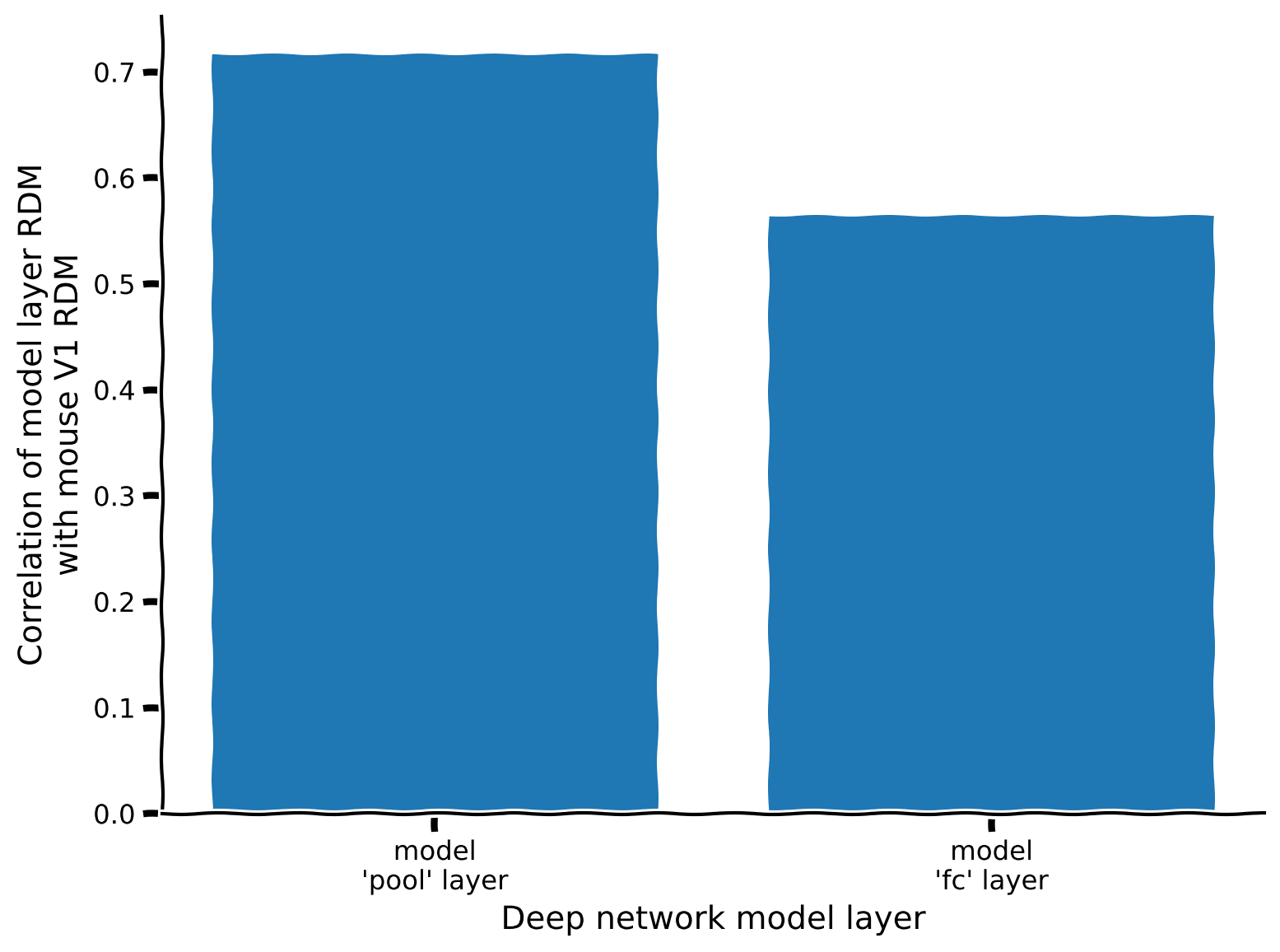
According to this metric, which layer’s representations most resemble those in the data? Does this agree with your intuitions from coding exercise 2.1?

Submit your feedback#

Section 2.3: Further understanding RDMs#

Estimated timing to here from start of tutorial: 45 min

To better understand how these correlations in RDM’s arise, we can try plotting individual rows of the RDM matrix. The resulting curves show the similarity of the responses to each stimulus with that to one specific stimulus.

ori_list = [-75, -25, 25, 75]
plot_rdm_rows(ori_list, rdm_dict, ori.numpy())

Section 3: Qualitative comparisons of CNNs and neural activity#

To visualize the representations in the data and in each of these model layers, we’ll use two classic techniques from systems neuroscience:

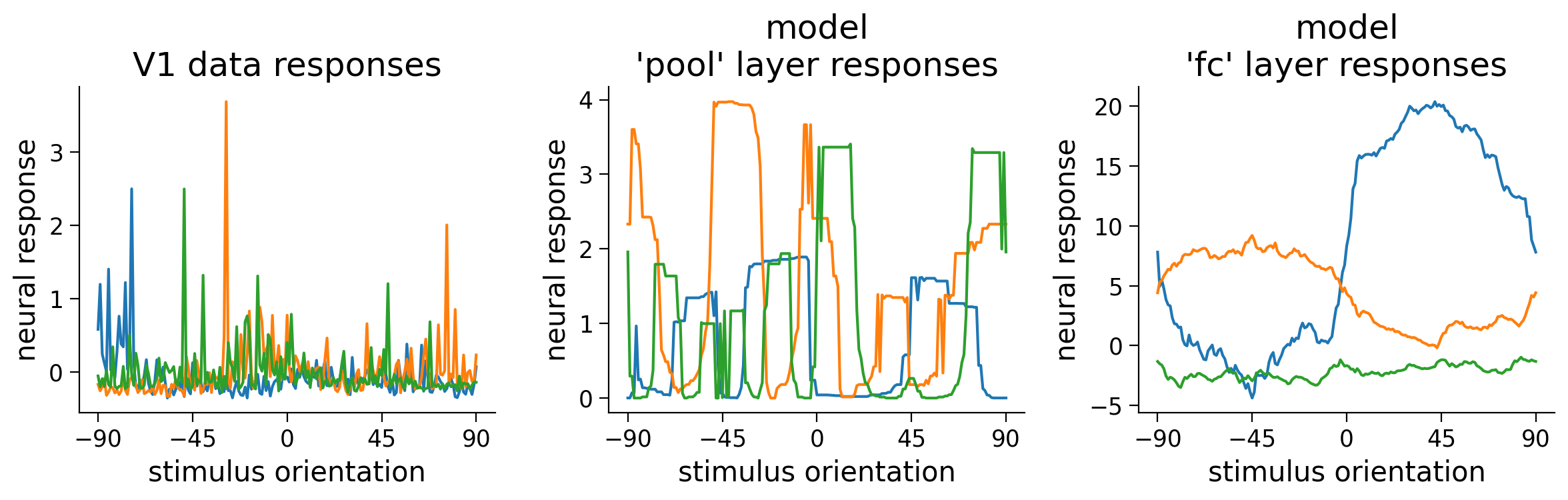
tuning curves: plotting the response of single neurons (or units, in the case of the deep network) as a function of the stimulus orientation
dimensionality reduction: plotting full population responses to each stimulus in two dimensions via dimensionality reduction. We’ll use the non-linear dimensionality reduction technique t-SNE for this. We use dimensionality reduction because there are many units and it’s difficult to visualize all of them at once. We use a non-linear dimensionality reduction technique because it can capture complex relationships between stimuli (see W1D5 for more details).

Section 3.1: Tuning Curves#

Estimated timing to here from start of tutorial: 50 min

Below, we show some example tuning curves for different neurons and units in the CNN we trained above. How are the single neuron responses similar/different between the model and the data? Try running this cell multiple times to get an idea of shared properties in the tuning curves of the neurons within each population.

Execute this cell to visualize tuning curves

../../../_images/4e73aead6f56180e8550dbd0b252ac7840281eb4803284db0fd60aee485b88d8.png

Section 3.2: Dimensionality reduction of representations#

Estimated timing to here from start of tutorial: 55 min

We can visualize a dimensionality-reduced version of the internal representations of the mouse primary visual cortex or CNN internal representations in order to potentially uncover informative structure. Here, we use PCA to reduce the dimensionality to 20 dimensions, and then use tSNE to further reduce dimensionality to 2 dimensions. We use the first step of PCA so that tSNE runs faster (this is standard practice in the field).

Execute this cell to visualize low-d representations

../../../_images/d75ff55929c44e0417549d412c0fb6a02fa92260925093b48391e958dcbb24f8.png

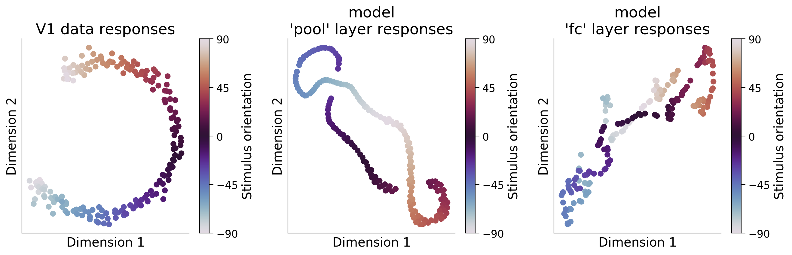
Think! 3.2: Visualizing reduced dimensionality representations#

Interpret the figure above. Why do these representations look the way they do? Here are a few specific questions to think about:

How are the population responses similar/different between the model and the data? Can you explain these population-level responses from the single neuron responses seen in the previous exercise, or vice-versa?
How do the representations in the different layers of the model differ, and how does this relate to the orientation discrimination task the model was optimized for?
Which layer of our deep network encoding model most closely resembles the V1 data?

Click for solution

Submit your feedback#

Summary#

Estimated timing of tutorial: 1 hour, 10 minutes

In this notebook, we learned

how to use deep learning to build a normative encoding model of the visual system
how to use RSA to evaluate how the model’s representations match to those in the brain

Our approach was to optimize a deep convolutional network to solve an orientation discrimination task. But note that many other approaches could have been taken.

Firstly, there are many other “normative” ways to solve this orientation discrimination task. We could have used different neural network architectures, or even used a completely different algorithm that didn’t involve a neural network at all, but instead used other kinds of image transformations (e.g. Fourier transforms). Neural network approaches, however, are special in that they explicitly use abstract distributed representations to compute, which feels a lot closer to the kinds of algorithms the brain uses. Convolutional neural networks in particular are well-suited for building normative models of the visual system.

Secondly, our choice of visual task was mostly arbitrary. For example, we could have trained our network to directly estimate the orientation of the stimulus, rather than just discriminating between two classes of tilt. Or, we could have trained the network to perform a more naturalistic task, such as recognizing the rotation of an arbitrary image. Or we could try a task like object recognition. Is this something that mice compute in their visual cortex?

Training on different tasks could lead to different representations of the oriented grating stimuli, which might match the observed V1 representations better or worse.

See Section 3 in the Bonus Tutorial to fit a convolutional neural network directly to neural activity to build an encoding model.

Bonus#

Bonus Section 1: Building CNN’s with PyTorch#

Here we walk through building the different types of layers in a CNN using PyTorch, culminating in the CNN model used above.

Bonus Section 1.1: Fully connected layers#

In a fully connected layer, each unit computes a weighted sum over all the input units and applies a non-linear function to this weighted sum. You have used such layers many times already in parts 1 and 2. As you have already seen, these are implemented in PyTorch using the nn.Linear class.

See the next cell for code for constructing a deep network with one fully connected layer that will classify an input image as being tilted left or right. Specifically, its output is the predicted probability of the input image being tilted right. To ensure that its output is a probability (i.e. a number between 0 and 1), we use a sigmoid activation function to squash the output into this range (implemented with torch.sigmoid()).

class FC(nn.Module):
  """Deep network with one fully connected layer

    Args:
      h_in (int): height of input image, in pixels (i.e. number of rows)
      w_in (int): width of input image, in pixels (i.e. number of columns)

    Attributes:
      fc (nn.Linear): weights and biases of fully connected layer
      out (nn.Linear): weights and biases of output layer

    """

  def __init__(self, h_in, w_in):
    super().__init__()
    self.dims = h_in * w_in  # dimensions of flattened input
    self.fc = nn.Linear(self.dims, 10)  # flattened input image --> 10D representation
    self.out = nn.Linear(10, 1)  # 10D representation --> scalar

  def forward(self, x):
    """Classify grating stimulus as tilted right or left

    Args:
      x (torch.Tensor): p x 48 x 64 tensor with pixel grayscale values for
          each of p stimulus images.

    Returns:
      torch.Tensor: p x 1 tensor with network outputs for each input provided
          in x. Each output should be interpreted as the probability of the
          corresponding stimulus being tilted right.

    """
    x = x.view(-1, self.dims)  # flatten each input image into a vector
    x = torch.relu(self.fc(x))  # output of fully connected layer
    x = torch.sigmoid(self.out(x))  # network output
    return x

Bonus Section 1.2: Convolutional layers#

In a convolutional layer, each unit computes a weighted sum over a two-dimensional \(K \times K\) patch of inputs. As we saw in part 2, the units are arranged in channels (see figure below), whereby units in the same channel compute the same weighted sum over different parts of the input, using the weights of that channel’s convolutional filter (or kernel). The output of a convolutional layer is thus a three-dimensional tensor of shape \(C^{out} \times H \times W\), where \(C^{out}\) is the number of channels (i.e. the number of convolutional filters/kernels), and \(H\) and \(W\) are the height and width of the input.

Such layers can be implemented in Python using the PyTorch class `nn.Conv2d as we saw in Tutorial 2 (documentation here).

See the next cell for code incorporating a convolutional layer with 8 convolutional filters of size 5 \(\times\) 5 into our above fully connected network. Note that we have to flatten the multi-channel output in order to pass it on to the fully connected layer.

class ConvFC(nn.Module):
  """Deep network with one convolutional layer and one fully connected layer

  Args:
    h_in (int): height of input image, in pixels (i.e. number of rows)
    w_in (int): width of input image, in pixels (i.e. number of columns)

  Attributes:
    conv (nn.Conv2d): filter weights of convolutional layer
    dims (tuple of ints): dimensions of output from conv layer
    fc (nn.Linear): weights and biases of fully connected layer
    out (nn.Linear): weights and biases of output layer

  """

  def __init__(self, h_in, w_in):
    super().__init__()
    C_in = 1  # input stimuli have only 1 input channel
    C_out = 6  # number of output channels (i.e. of convolutional kernels to convolve the input with)
    K = 7  # size of each convolutional kernel (should be odd number for the padding to work as expected)
    self.conv = nn.Conv2d(C_in, C_out, kernel_size=K, padding=K//2)  # add padding to ensure that each channel has same dimensionality as input
    self.dims = (C_out, h_in, w_in)  # dimensions of conv layer output
    self.fc = nn.Linear(np.prod(self.dims), 10)  # flattened conv output --> 10D representation
    self.out = nn.Linear(10, 1)  # 10D representation --> scalar

  def forward(self, x):
    """Classify grating stimulus as tilted right or left

    Args:
      x (torch.Tensor): p x 48 x 64 tensor with pixel grayscale values for
          each of p stimulus images.

    Returns:
      torch.Tensor: p x 1 tensor with network outputs for each input provided
          in x. Each output should be interpreted as the probability of the
          corresponding stimulus being tilted right.

    """
    x = x.unsqueeze(1)  # p x 1 x 48 x 64, add a singleton dimension for the single stimulus channel
    x = torch.relu(self.conv(x))  # output of convolutional layer
    x = x.view(-1, np.prod(self.dims))  # flatten convolutional layer outputs into a vector
    x = torch.relu(self.fc(x))  # output of fully connected layer
    x = torch.sigmoid(self.out(x))  # network output
    return x

Bonus Section 1.3: Max pooling layers#

In a max pooling layer, each unit computes the maximum over a small two-dimensional \(K^{pool} \times K^{pool}\) patch of inputs. Given a multi-channel input of dimensions \(C \times H \times W\), the output of a max pooling layer has dimensions \(C \times H^{out} \times W^{out}\), where:

(245)#\[\begin{align} H^{out} &= \left\lfloor \frac{H}{K^{pool}} \right\rfloor\\ W^{out} &= \left\lfloor \frac{W}{K^{pool}} \right\rfloor \end{align}\]

where \(\lfloor\cdot\rfloor\) denotes rounding down to the nearest integer below (i.e., floor division // in Python).

Max pooling layers can be implemented with the PyTorch nn.MaxPool2d class, which takes as a single argument the size \(K^{pool}\) of the pooling patch. See the next cell for an example, which builds upon the previous example by adding in a max pooling layer just after the convolutional layer. Note again that we need to calculate the dimensions of its output in order to set the dimensions of the subsequent fully connected layer.

class ConvPoolFC(nn.Module):
  """Deep network with one convolutional layer followed by a max pooling layer
  and one fully connected layer

  Args:
    h_in (int): height of input image, in pixels (i.e. number of rows)
    w_in (int): width of input image, in pixels (i.e. number of columns)

  Attributes:
    conv (nn.Conv2d): filter weights of convolutional layer
    pool (nn.MaxPool2d): max pooling layer
    dims (tuple of ints): dimensions of output from pool layer
    fc (nn.Linear): weights and biases of fully connected layer
    out (nn.Linear): weights and biases of output layer

  """

  def __init__(self, h_in, w_in):
    super().__init__()
    C_in = 1  # input stimuli have only 1 input channel
    C_out = 6  # number of output channels (i.e. of convolutional kernels to convolve the input with)
    K = 7  # size of each convolutional kernel
    Kpool = 8  # size of patches over which to pool
    self.conv = nn.Conv2d(C_in, C_out, kernel_size=K, padding=K//2)  # add padding to ensure that each channel has same dimensionality as input
    self.pool = nn.MaxPool2d(Kpool)
    self.dims = (C_out, h_in // Kpool, w_in // Kpool)  # dimensions of pool layer output
    self.fc = nn.Linear(np.prod(self.dims), 10)  # flattened pool output --> 10D representation
    self.out = nn.Linear(10, 1)  # 10D representation --> scalar

  def forward(self, x):
    """Classify grating stimulus as tilted right or left

    Args:
      x (torch.Tensor): p x 48 x 64 tensor with pixel grayscale values for
          each of p stimulus images.

    Returns:
      torch.Tensor: p x 1 tensor with network outputs for each input provided
          in x. Each output should be interpreted as the probability of the
          corresponding stimulus being tilted right.

    """
    x = x.unsqueeze(1)  # p x 1 x 48 x 64, add a singleton dimension for the single stimulus channel
    x = torch.relu(self.conv(x))  # output of convolutional layer
    x = self.pool(x)  # output of pooling layer
    x = x.view(-1, np.prod(self.dims))  # flatten pooling layer outputs into a vector
    x = torch.relu(self.fc(x))  # output of fully connected layer
    x = torch.sigmoid(self.out(x))  # network output
    return x

This pooling layer completes the CNN model trained above to perform orientation discrimination. We can think of this architecture as having two primary layers:

a convolutional + pooling layer
a fully connected layer

We group together the convolution and pooling layers into one, as they really form one full unit of convolutional processing, where each patch of the image is passed through a convolutional filter and pooled with neighboring patches. It is standard practice to follow up any convolutional layer with a pooling layer, so they are generally treated as a single block of processing.

Bonus Section 2: Orientation discrimination as a binary classification problem#

What loss function should we minimize to optimize orientation discrimination performance? We first note that the orientation discrimination task is a binary classification problem, where the goal is to classify a given stimulus into one of two classes: being tilted left or being tilted right.

Our goal is thus to output a high probability of the stimulus being tilted right (i.e. large \(p\)) whenever the stimulus is tilted right, and a high probability of the stimulus being tilted left (i.e. large \(1-p \Leftrightarrow\) small \(p\)) whenever the stimulus is tilted left.

Let \(\tilde{y}^{(n)}\) be the label of the \(n\)th stimulus in the mini-batch, indicating its true tilt:

(246)#\[\begin{equation} \tilde{y}^{(n)} = \begin{cases} 1 &\text{if stimulus }n\text{ is tilted right} \\ 0 &\text{if stimulus }n\text{ is tilted left} \end{cases} \end{equation}\]

Let \(p^{(n)}\) be the predicted probability of that stimulus being tilted right assigned by our network. Note that that \(1-p^{(n)}\) is the predicted probability of that stimulus being tilted left. We’d now like to modify the parameters so as to maximize the predicted probability of the true class \(\tilde{y}^{(n)}\). One way to formalize this is as maximizing the log probability

(247)#\[\begin{align} \log \left( \text{predicted probability of stimulus } n \text{ being of class } \tilde{y}^{(n)}\right) &= \begin{cases} \log p^{(n)} &\text{if }\tilde{y}^{(n)} = 1 \\ \log (1 - p^{(n)}) &\text{if }\tilde{y}^{(n)} = 0 \end{cases} \\ &= \tilde{y}^{(n)} \log p^{(n)} + (1 - \tilde{y}^{(n)})\log(1 - p^{(n)}) \end{align}\]

You should recognize this expression as the log likelihood of the Bernoulli distribution under the predicted probability \(p^{(n)}\). This is the same quantity that is maximized in logistic regression, where the predicted probability \(p^{(n)}\) is just a simple linear sum of its inputs (rather than a complicated non-linear operation, like in the deep networks used here).

To turn this into a loss function, we simply multiply it by -1, resulting in the so-called binary cross-entropy, or negative log likelihood. Summing over \(P\) samples in a batch, the binary cross entropy loss is given by

(248)#\[\begin{equation} L = -\sum_{n=1}^P \tilde{y}^{(n)} \log p^{(n)} + (1 - \tilde{y}^{(n)})\log(1 - p^{(n)}) \end{equation}\]

The binary cross-entropy loss can be implemented in PyTorch using the nn.BCELoss() loss function (cf. documentation).

Feel free to check out the code used to optimize the CNN in the train() function defined in the hidden cell of helper functions at the top of the notebook. Because the CNN’s used here have lots of parameters, we have to use two tricks that we didn’t use in the previous parts of this tutorial:

We have to use stochastic gradient descent (SGD), rather than just gradient descent (GD).
We have to use momentum in our SGD updates. This is easily incorporated into our PyTorch implementation by just setting the momentum argument of the built-in optim.SGD optimizer.

Bonus Section 3: RDM Z-Score Explanation#

If \(r^{(s)}_i\) is the response of the \(i\)-th neuron to the \(s\)-th stimulus, then

(249)#\[\begin{gather} M_{ss'} = 1 - \frac{\text{Cov}\left[ r_i^{(s)}, r_i^{(s')} \right]}{\sqrt{\text{Var}\left[ r_i^{(s)} \right] \text{Var}\left[ r_i^{(s')} \right]}} = 1 - \frac{\sum_{i=1}^N (r_i^{(s)} - \bar{r}^{(s)})(r_i^{(s')} - \bar{r}^{(s')}) }{\sqrt{\sum_{i=1}^N \left( r_i^{(s)} - \bar{r}^{(s)} \right)^2 \sum_{i=1}^N \left( r_i^{(s')} - \bar{r}^{(s')} \right)^2 }} \\ \bar{r}^{(s)} = \frac{1}{N} \sum_{i=1}^N r_i^{(s)} \end{gather}\]

This can be computed efficiently by using the \(z\)-scored responses

(250)#\[\begin{equation} z_i^{(s)} = \frac{r_i^{(s)} - \bar{r}^{(s)}}{\sqrt{\frac{1}{N}\sum_{i=1}^N \left( r_i^{(s)} - \bar{r}^{(s)} \right)^2}} \Rightarrow M_{ss'} = 1 - \frac{1}{N}\sum_{i=1}^N z_i^{(s)}z_i^{(s')} \end{equation}\]

such that the full matrix can be computed through the matrix multiplication

(251)#\[\begin{gather} \mathbf{M} = 1 - \frac{1}{N} \mathbf{ZZ}^\top \\ \mathbf{Z} = \begin{bmatrix} z_1^{(1)} & z_2^{(1)} & \ldots & z_N^{(1)} \\ z_1^{(2)} & z_2^{(2)} & \ldots & z_N^{(2)} \\ \vdots & \vdots & \ddots & \vdots \\ z_1^{(S)} & z_2^{(S)} & \ldots & z_N^{(S)} \end{bmatrix} \end{gather}\]

where \(S\) is the total number of stimuli. Note that \(\mathbf{Z}\) is an \(S \times N\) matrix, and \(\mathbf{M}\) is an \(S \times S\) matrix.

Tutorial 3: Building and Evaluating Normative Encoding Models

Contents

Tutorial 3: Building and Evaluating Normative Encoding Models#

Tutorial Objectives#

Setup#

Install and import feedback gadget#

Figure Settings#

Plotting Functions#

Helper Functions#

Data retrieval and loading#

Section 1: Setting up deep network and neural data#

Video 1: Deep convolutional network for orientation discrimination#

Submit your feedback#

Section 1.1: Orientation discrimination task#

Section 1.2: A deep network model of orientation discrimination#

Section 1.3: Load data#

Section 2: Quantitative comparisons of CNNs and neural activity#

Video 2: Quantitative comparisons of CNNs and neural activity#

Submit your feedback#

Section 2.1: Representational dissimilarity matrix (RDM)#

Coding Exercise 2.1: Compute RDMs#

Submit your feedback#

Video 3: Coding Exercise 2.1 solution discussion#

Submit your feedback#

Section 2.2: Determining representation similarity#

Coding Exercise 2.2: Correlate RDMs#

Submit your feedback#

Section 2.3: Further understanding RDMs#

Section 3: Qualitative comparisons of CNNs and neural activity#

Section 3.1: Tuning Curves#

Section 3.2: Dimensionality reduction of representations#

Think! 3.2: Visualizing reduced dimensionality representations#

Submit your feedback#

Summary#

Bonus#

Bonus Section 1: Building CNN’s with PyTorch#

Bonus Section 1.1: Fully connected layers#

Bonus Section 1.2: Convolutional layers#

Bonus Section 1.3: Max pooling layers#

Bonus Section 2: Orientation discrimination as a binary classification problem#

Bonus Section 3: RDM Z-Score Explanation#