Tutorial 1: Geometric view of data

Tutorial 1: Geometric view of data#

Week 1, Day 4: Dimensionality Reduction

By Neuromatch Academy

Content creators: Alex Cayco Gajic, John Murray

Content reviewers: Roozbeh Farhoudi, Matt Krause, Spiros Chavlis, Richard Gao, Michael Waskom, Siddharth Suresh, Natalie Schaworonkow, Ella Batty

Production editors: Gagana B, Spiros Chavlis

Tutorial Objectives#

Estimated timing of tutorial: 50 minutes

In this notebook we’ll explore how multivariate data can be represented in different orthonormal bases. This will help us build intuition that will be helpful in understanding PCA in the following tutorial.

Overview:

Generate correlated multivariate data.
Define an arbitrary orthonormal basis.
Project the data onto the new basis.

Setup#

Install and import feedback gadget#

# Imports
import numpy as np
import matplotlib.pyplot as plt

Figure Settings#

Plotting Functions#

Show code cell source Hide code cell source

# @title Plotting Functions

def plot_data(X):
  """
  Plots bivariate data. Includes a plot of each random variable, and a scatter
  plot of their joint activity. The title indicates the sample correlation
  calculated from the data.

  Args:
    X (numpy array of floats) : Data matrix each column corresponds to a
                                different random variable

  Returns:
    Nothing.
  """

  fig = plt.figure(figsize=[8, 4])
  gs = fig.add_gridspec(2, 2)
  ax1 = fig.add_subplot(gs[0, 0])
  ax1.plot(X[:, 0], color='k')
  plt.ylabel('Neuron 1')
  plt.title(f'Sample var 1: {np.var(X[:, 0]):.1f}')
  ax1.set_xticklabels([])
  ax2 = fig.add_subplot(gs[1, 0])
  ax2.plot(X[:, 1], color='k')
  plt.xlabel('Sample Number')
  plt.ylabel('Neuron 2')
  plt.title(f'Sample var 2: {np.var(X[:, 1]):.1f}')
  ax3 = fig.add_subplot(gs[:, 1])
  ax3.plot(X[:, 0], X[:, 1], '.', markerfacecolor=[.5, .5, .5],
           markeredgewidth=0)
  ax3.axis('equal')
  plt.xlabel('Neuron 1 activity')
  plt.ylabel('Neuron 2 activity')
  plt.title(f'Sample corr: {np.corrcoef(X[:, 0], X[:, 1])[0, 1]:.1f}')
  plt.show()


def plot_basis_vectors(X, W):
  """
  Plots bivariate data as well as new basis vectors.

  Args:
    X (numpy array of floats) : Data matrix each column corresponds to a
                                different random variable
    W (numpy array of floats) : Square matrix representing new orthonormal
                                basis each column represents a basis vector

  Returns:
    Nothing.
  """

  plt.figure(figsize=[4, 4])
  plt.plot(X[:, 0], X[:, 1], '.', color=[.5, .5, .5], label='Data')
  plt.axis('equal')
  plt.xlabel('Neuron 1 activity')
  plt.ylabel('Neuron 2 activity')
  plt.plot([0, W[0, 0]], [0, W[1, 0]], color='r', linewidth=3,
           label='Basis vector 1')
  plt.plot([0, W[0, 1]], [0, W[1, 1]], color='b', linewidth=3,
           label='Basis vector 2')
  plt.legend()
  plt.show()


def plot_data_new_basis(Y):
  """
  Plots bivariate data after transformation to new bases.
  Similar to plot_data but with colors corresponding to projections onto
  basis 1 (red) and basis 2 (blue). The title indicates the sample correlation
  calculated from the data.

  Note that samples are re-sorted in ascending order for the first
  random variable.

  Args:
    Y (numpy array of floats) : Data matrix in new basis each column
                                corresponds to a different random variable

  Returns:
    Nothing.
  """
  fig = plt.figure(figsize=[8, 4])
  gs = fig.add_gridspec(2, 2)
  ax1 = fig.add_subplot(gs[0, 0])
  ax1.plot(Y[:, 0], 'r')
  plt.xlabel
  plt.ylabel('Projection \n basis vector 1')
  plt.title(f'Sample var 1: {np.var(Y[:, 0]):.1f}')
  ax1.set_xticklabels([])
  ax2 = fig.add_subplot(gs[1, 0])
  ax2.plot(Y[:, 1], 'b')
  plt.xlabel('Sample number')
  plt.ylabel('Projection \n basis vector 2')
  plt.title(f'Sample var 2: {np.var(Y[:, 1]):.1f}')
  ax3 = fig.add_subplot(gs[:, 1])
  ax3.plot(Y[:, 0], Y[:, 1], '.', color=[.5, .5, .5])
  ax3.axis('equal')
  plt.xlabel('Projection basis vector 1')
  plt.ylabel('Projection basis vector 2')
  plt.title(f'Sample corr: {np.corrcoef(Y[:, 0], Y[:, 1])[0, 1]:.1f}')
  plt.show()

Video 1: Geometric view of data#

Submit your feedback#

Section 1: Generate correlated multivariate data#

Video 2: Multivariate data#

This video describes the covariance matrix and the multivariate normal distribution.

Click here for text recap of video

To gain intuition, we will first use a simple model to generate multivariate data. Specifically, we will draw random samples from a bivariate normal distribution. This is an extension of the one-dimensional normal distribution to two dimensions, in which each \(x_i\) is marginally normal with mean \(\mu_i\) and variance \(\sigma_i^2\):

(202)#\[\begin{equation} x_i \sim \mathcal{N}(\mu_i,\sigma_i^2). \end{equation}\]

Additionally, the joint distribution for \(x_1\) and \(x_2\) has a specified correlation coefficient \(\rho\). Recall that the correlation coefficient is a normalized version of the covariance, and ranges between -1 and +1:

(203)#\[\begin{equation} \rho = \frac{\text{cov}(x_1, x_2)}{\sqrt{\sigma_1^2 \sigma_2^2}}. \end{equation}\]

For simplicity, we will assume that the mean of each variable has already been subtracted, so that \(\mu_i=0\) for both \(i=1\) and \(i=2\). The remaining parameters can be summarized in the covariance matrix, which for two dimensions has the following form:

(204)#\[\begin{equation} {\bf \Sigma} = \begin{pmatrix} \text{var}(x_1) & \text{cov}(x_1,x_2) \\ \text{cov}(x_1,x_2) &\text{var}(x_2) \end{pmatrix}. \end{equation}\]

In general, \(\bf \Sigma\) is a symmetric matrix with the variances \(\text{var}(x_i) = \sigma_i^2\) on the diagonal, and the covariances on the off-diagonal. Later, we will see that the covariance matrix plays a key role in PCA.

Submit your feedback#

Coding Exercise 1: Draw samples from a distribution#

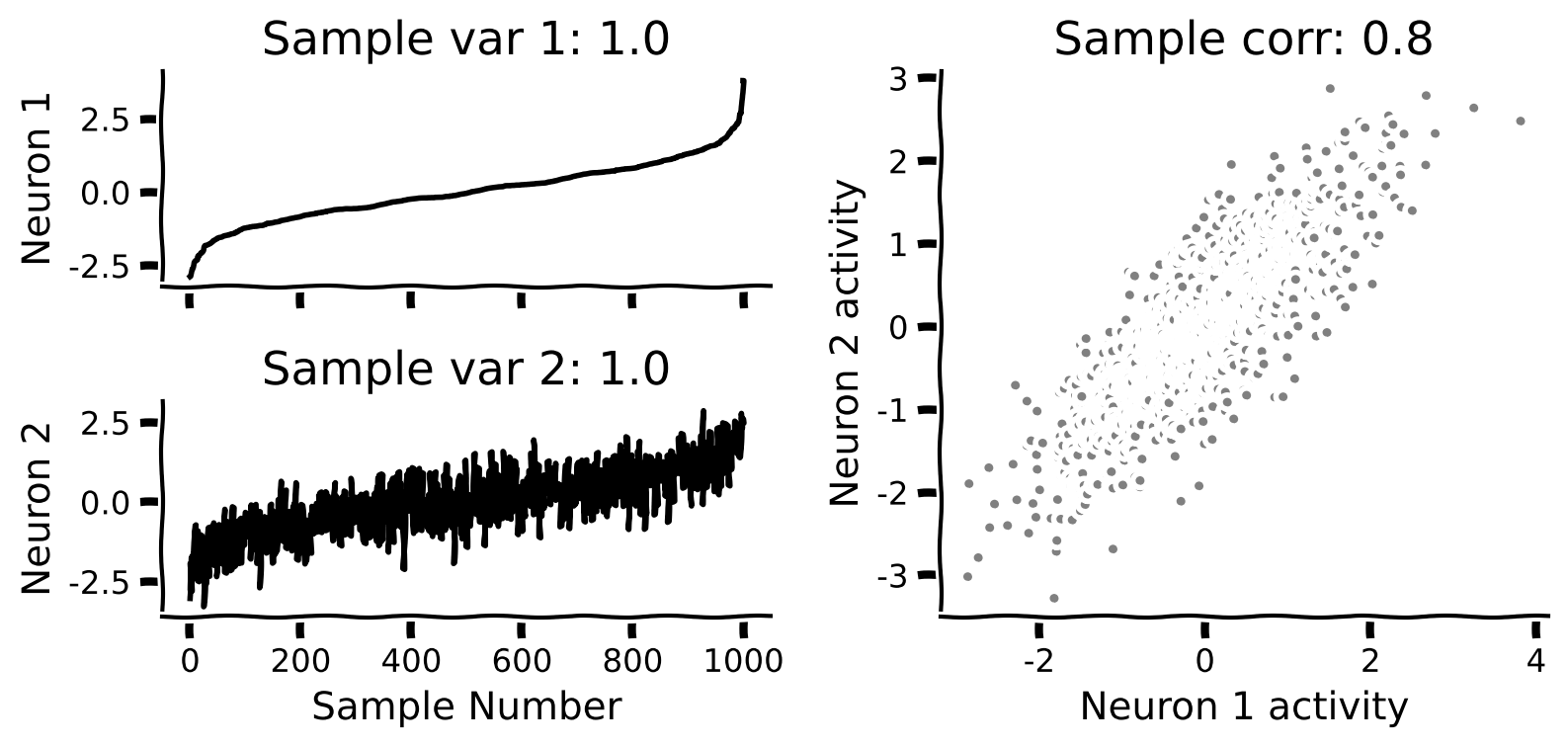
We have provided code to draw random samples from a zero-mean bivariate normal distribution with a specified covariance matrix (get_data). Throughout this tutorial, we’ll imagine these samples represent the activity (firing rates) of two recorded neurons on different trials. Fill in the function below to calculate the covariance matrix given the desired variances and correlation coefficient. The covariance can be found by rearranging the equation above:

(205)#\[\begin{equation} \text{cov}(x_1,x_2) = \rho \sqrt{\sigma_1^2 \sigma_2^2}. \end{equation}\]

Execute this cell to get helper function get_data

Help on function get_data in module __main__:

get_data(cov_matrix)
    Returns a matrix of 1000 samples from a bivariate, zero-mean Gaussian.
    
    Note that samples are sorted in ascending order for the first random variable
    
    Args:
      cov_matrix (numpy array of floats): desired covariance matrix
    
    Returns:
      (numpy array of floats) : samples from the bivariate Gaussian, with each
                                column corresponding to a different random
                                variable

def calculate_cov_matrix(var_1, var_2, corr_coef):
  """
  Calculates the covariance matrix based on the variances and correlation
  coefficient.

  Args:
    var_1 (scalar)          : variance of the first random variable
    var_2 (scalar)          : variance of the second random variable
    corr_coef (scalar)      : correlation coefficient

  Returns:
    (numpy array of floats) : covariance matrix
  """

  #################################################
  ## TODO for students: calculate the covariance matrix
  # Fill out function and remove
  raise NotImplementedError("Student exercise: calculate the covariance matrix!")
  #################################################

  # Calculate the covariance from the variances and correlation
  cov = ...

  cov_matrix = np.array([[var_1, cov], [cov, var_2]])

  return cov_matrix


# Set parameters
np.random.seed(2020)  # set random seed
variance_1 = 1
variance_2 = 1
corr_coef = 0.8

# Compute covariance matrix
cov_matrix = calculate_cov_matrix(variance_1, variance_2, corr_coef)

# Generate data with this covariance matrix
X = get_data(cov_matrix)

# Visualize
plot_data(X)

Click for solution

Example output:

Submit your feedback#

Interactive Demo 1: Correlation effect on data#

We’ll use the function you just completed but now we can change the correlation coefficient via slider. You should get a feel for how changing the correlation coefficient affects the geometry of the simulated data.

What effect do negative correlation coefficient values have?
What correlation coefficient results in a circular data cloud?

Note that we sort the samples according to neuron 1’s firing rate, meaning the plot of neuron 1 firing rate over sample number looks clean and pretty unchanging when compared to neuron 2.

Execute this cell to enable widget

Click for solution

Submit your feedback#

Section 2: Define a new orthonormal basis#

Estimated timing to here from start of tutorial: 20 min

Video 3: Orthonormal bases#

Submit your feedback#

This video shows that data can be represented in many ways using different bases. It also explains how to check if your favorite basis is orthonormal.

Click here for text recap of video

Next, we will define a new orthonormal basis of vectors \({\bf u} = [u_1,u_2]\) and \({\bf w} = [w_1,w_2]\). As we learned in the video, two vectors are orthonormal if:

They are orthogonal (i.e., their dot product is zero):

(206)#\[\begin{equation} {\bf u\cdot w} = u_1 w_1 + u_2 w_2 = 0 \end{equation}\]

They have unit length:

(207)#\[\begin{equation} ||{\bf u}|| = ||{\bf w} || = 1 \end{equation}\]

In two dimensions, it is easy to make an arbitrary orthonormal basis. All we need is a random vector \({\bf u}\), which we have normalized. If we now define the second basis vector to be \({\bf w} = [-u_2,u_1]\), we can check that both conditions are satisfied:

(208)#\[\begin{equation} {\bf u\cdot w} = - u_1 u_2 + u_2 u_1 = 0 \end{equation}\]

and

(209)#\[\begin{equation} {|| {\bf w} ||} = \sqrt{(-u_2)^2 + u_1^2} = \sqrt{u_1^2 + u_2^2} = 1, \end{equation}\]

where we used the fact that \({\bf u}\) is normalized. So, with an arbitrary input vector, we can define an orthonormal basis, which we will write in matrix by stacking the basis vectors horizontally:

(210)#\[\begin{equation} {{\bf W} } = \begin{pmatrix} u_1 & w_1 \\ u_2 & w_2 \end{pmatrix}. \end{equation}\]

Coding Exercise 2: Find an orthonormal basis#

In this exercise you will fill in the function below to define an orthonormal basis, given a single arbitrary 2-dimensional vector as an input.

Steps

Modify the function define_orthonormal_basis to first normalize the first basis vector \(\bf u\).
Then complete the function by finding a basis vector \(\bf w\) that is orthogonal to \(\bf u\).
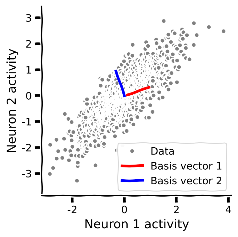
Test the function using initial basis vector \({\bf u} = [3,1]\). Plot the resulting basis vectors on top of the data scatter plot using the function plot_basis_vectors. (For the data, use \(\sigma_1^2 =1\), \(\sigma_2^2 =1\), and \(\rho = .8\)).

def define_orthonormal_basis(u):
  """
  Calculates an orthonormal basis given an arbitrary vector u.

  Args:
    u (numpy array of floats) : arbitrary 2-dimensional vector used for new
                                basis

  Returns:
    (numpy array of floats)   : new orthonormal basis
                                columns correspond to basis vectors
  """

  #################################################
  ## TODO for students: calculate the orthonormal basis
  # Fill out function and remove
  raise NotImplementedError("Student exercise: implement the orthonormal basis function")
  #################################################

  # Normalize vector u
  u = ...

  # Calculate vector w that is orthogonal to u
  w = ...

  # Put in matrix form
  W = np.column_stack([u, w])

  return W


# Set up parameters
np.random.seed(2020)  # set random seed
variance_1 = 1
variance_2 = 1
corr_coef = 0.8
u = np.array([3, 1])

# Compute covariance matrix
cov_matrix = calculate_cov_matrix(variance_1, variance_2, corr_coef)

# Generate data
X = get_data(cov_matrix)

# Get orthonomal basis
W = define_orthonormal_basis(u)

# Visualize
plot_basis_vectors(X, W)

Click for solution

Example output:

Submit your feedback#

Section 3: Project data onto new basis#

Estimated timing to here from start of tutorial: 35 min

Video 4: Change of basis#

Submit your feedback#

Finally, we will express our data in the new basis that we have just found. Since \(\bf W\) is orthonormal, we can project the data into our new basis using simple matrix multiplication :

(211)#\[\begin{equation} {\bf Y = X W}. \end{equation}\]

We will explore the geometry of the transformed data \(\bf Y\) as we vary the choice of basis.

Coding Exercise 3: Change to orthonormal basis#

In this exercise you will fill in the function below to change data to an orthonormal basis.

Steps

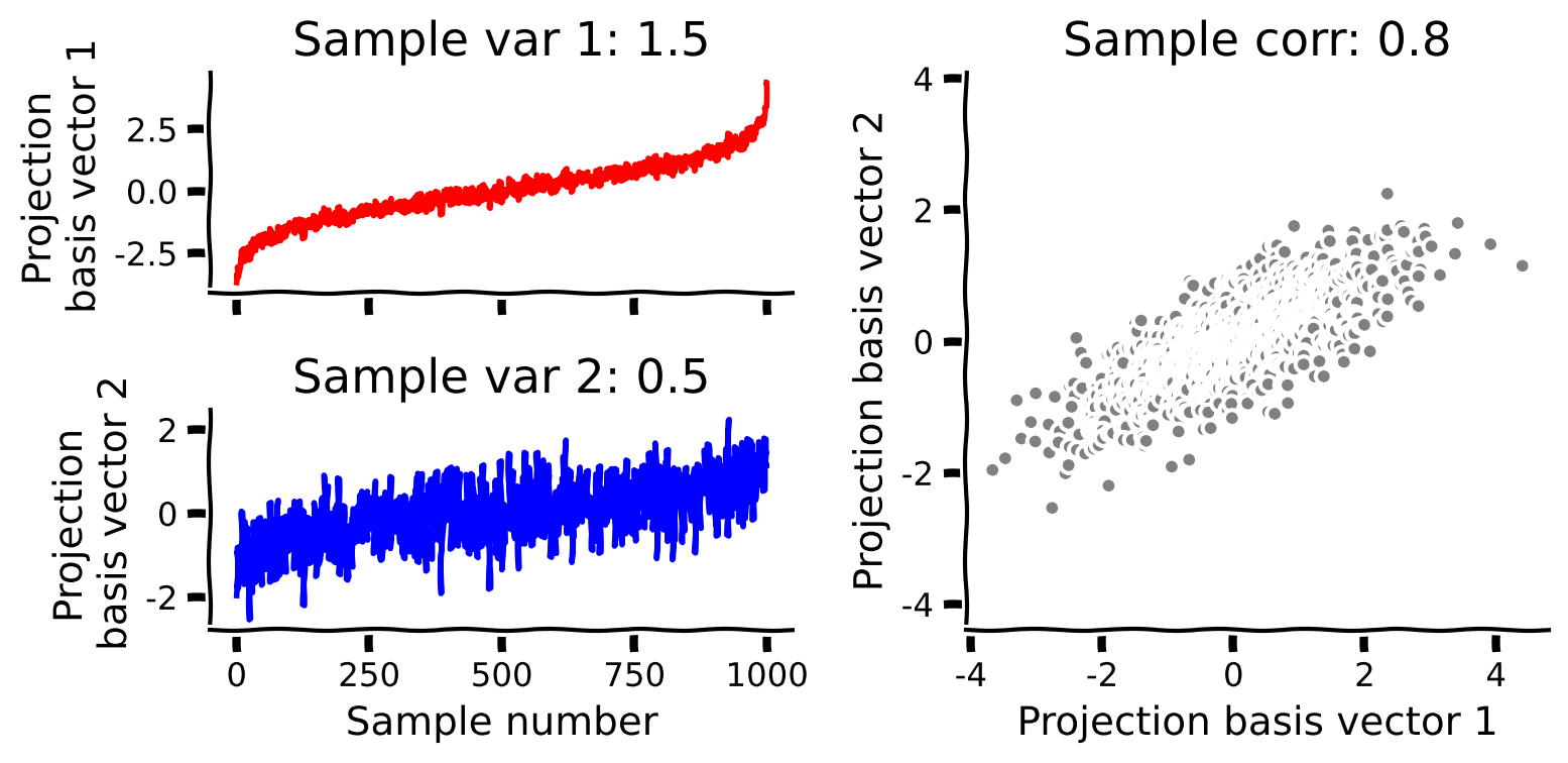
Complete the function change_of_basis to project the data onto the new basis.
Plot the projected data using the function plot_data_new_basis.
What happens to the correlation coefficient in the new basis? Does it increase or decrease?
What happens to variance?

def change_of_basis(X, W):
  """
  Projects data onto new basis W.

  Args:
    X (numpy array of floats) : Data matrix each column corresponding to a
                                different random variable
    W (numpy array of floats) : new orthonormal basis columns correspond to
                                basis vectors

  Returns:
    (numpy array of floats)    : Data matrix expressed in new basis
  """

  #################################################
  ## TODO for students: project the data onto a new basis W
  # Fill out function and remove
  raise NotImplementedError("Student exercise: implement change of basis")
  #################################################

  # Project data onto new basis described by W
  Y = ...

  return Y


# Project data to new basis
Y = change_of_basis(X, W)

# Visualize
plot_data_new_basis(Y)

Click for solution

Example output:

Submit your feedback#

Interactive Demo 3: Play with the basis vectors#

To see what happens to the correlation as we change the basis vectors, run the cell below. The parameter \(\theta\) controls the angle of \(\bf u\) in degrees. Use the slider to rotate the basis vectors.

What happens to the projected data as you rotate the basis?
How does the correlation coefficient change? How does the variance of the projection onto each basis vector change?
Are you able to find a basis in which the projected data is uncorrelated?

Make sure you execute this cell to enable the widget!

Click for solution

Submit your feedback#

Summary#

Estimated timing of tutorial: 50 minutes

In this tutorial, we learned that multivariate data can be visualized as a cloud of points in a high-dimensional vector space. The geometry of this cloud is shaped by the covariance matrix.
Multivariate data can be represented in a new orthonormal basis using the dot product. These new basis vectors correspond to specific mixtures of the original variables - for example, in neuroscience, they could represent different ratios of activation across a population of neurons.
The projected data (after transforming into the new basis) will generally have a different geometry from the original data. In particular, taking basis vectors that are aligned with the spread of cloud of points decorrelates the data.

These concepts - covariance, projections, and orthonormal bases - are key for understanding PCA, which will be our focus in the next tutorial.

Notation#

(212)#\[\begin{align} x_i &\quad \text{data point for dimension } i\\ \mu_i &\quad \text{mean along dimension } i\\ \sigma_i^2 &\quad \text{variance along dimension } i \\ \bf u, \bf w &\quad \text{orthonormal basis vectors}\\ \rho &\quad \text{correlation coefficient}\\ \bf \Sigma &\quad \text{covariance matrix}\\ \bf X &\quad \text{original data matrix}\\ \bf W &\quad \text{projection matrix}\\ \bf Y &\quad \text{transformed data}\\ \end{align}\]

Tutorial 1: Geometric view of data

Contents

Tutorial 1: Geometric view of data#

Tutorial Objectives#

Setup#

Install and import feedback gadget#

Figure Settings#

Plotting Functions#

Video 1: Geometric view of data#

Submit your feedback#

Section 1: Generate correlated multivariate data#

Video 2: Multivariate data#

Submit your feedback#

Coding Exercise 1: Draw samples from a distribution#

Submit your feedback#

Interactive Demo 1: Correlation effect on data#

Submit your feedback#

Section 2: Define a new orthonormal basis#

Video 3: Orthonormal bases#

Submit your feedback#

Coding Exercise 2: Find an orthonormal basis#

Submit your feedback#

Section 3: Project data onto new basis#

Video 4: Change of basis#

Submit your feedback#

Coding Exercise 3: Change to orthonormal basis#

Submit your feedback#

Interactive Demo 3: Play with the basis vectors#

Submit your feedback#

Summary#

Notation#