![]()

Tutorial 1: Linear dynamical systems#
Week 2, Day 2: Linear Systems
By Neuromatch Academy
Content Creators: Bing Wen Brunton, Alice Schwarze
Content Reviewers: Norma Kuhn, Karolina Stosio, John Butler, Matthew Krause, Ella Batty, Richard Gao, Michael Waskom
Production editors: Gagana B, Spiros Chavlis
Tutorial Objectives#
Estimated timing of tutorial: 1 hour
In this tutorial, we will be learning about behavior of dynamical systems – systems that evolve in time – where the rules by which they evolve in time are described precisely by a differential equation.
Differential equations are equations that express the rate of change of the state variable \(x\). One typically describes this rate of change using the derivative of \(x\) with respect to time (\(dx/dt\)) on the left hand side of the differential equation:
A common notational short-hand is to write \(\dot{x}\) for \(\frac{dx}{dt}\). The dot means “the derivative with respect to time”.
Today, the focus will be on linear dynamics, where \(f(x)\) is a linear function of \(x\). In Tutorial 1, we will:
Explore and understand the behavior of such systems where \(x\) is a single variable
Consider cases where \(\mathbf{x}\) is a state vector representing two variables.
Setup#
Install and import feedback gadget#
Show code cell source
# @title Install and import feedback gadget

!pip3 install vibecheck datatops --quiet

from vibecheck import DatatopsContentReviewContainer
def content_review(notebook_section: str):
    return DatatopsContentReviewContainer(
        "",  # No text prompt
        notebook_section,
        {
            "url": "https://pmyvdlilci.execute-api.us-east-1.amazonaws.com/klab",
            "name": "neuromatch_cn",
            "user_key": "y1x3mpx5",
        },
    ).render()


feedback_prefix = "W2D2_T1"
# Imports
import numpy as np
import matplotlib.pyplot as plt
from scipy.integrate import solve_ivp  # numerical integration solver
Figure settings#
Show code cell source
# @title Figure settings
import logging
logging.getLogger('matplotlib.font_manager').disabled = True

import ipywidgets as widgets  # interactive display
%config InlineBackend.figure_format = 'retina'
plt.style.use("https://raw.githubusercontent.com/NeuromatchAcademy/course-content/main/nma.mplstyle")
Plotting Functions#
Show code cell source
# @title Plotting Functions
def plot_trajectory(system, params, initial_condition, dt=0.1, T=6,
                    figtitle=None):

  """
  Shows the solution of a linear system with two variables in 3 plots.
  The first plot shows x1 over time. The second plot shows x2 over time.
  The third plot shows x1 and x2 in a phase portrait.

  Args:
    system (function): a function f(x) that computes a derivative from
                        inputs (t, [x1, x2], *params)
    params (list or tuple): list of parameters for function "system"
    initial_condition (list or array): initial condition x0
    dt (float): time step of simulation
    T (float): end time of simulation
    figtitlte (string): title for the figure

  Returns:
    nothing, but it shows a figure
  """

  # time points for which we want to evaluate solutions
  t = np.arange(0, T, dt)

  # Integrate
  # use built-in ode solver
  solution = solve_ivp(system,
                    t_span=(0, T),
                    y0=initial_condition, t_eval=t,
                    args=(params),
                    dense_output=True)
  x = solution.y

  # make a color map to visualize time
  timecolors = np.array([(1 , 0 , 0, i)  for i in t / t[-1]])

  # make a large figure
  fig, (ah1, ah2, ah3) = plt.subplots(1, 3)
  fig.set_size_inches(10, 3)

  # plot x1 as a function of time
  ah1.scatter(t, x[0,], color=timecolors)
  ah1.set_xlabel('time')
  ah1.set_ylabel('x1', labelpad=-5)

  # plot x2 as a function of time
  ah2.scatter(t, x[1], color=timecolors)
  ah2.set_xlabel('time')
  ah2.set_ylabel('x2', labelpad=-5)

  # plot x1 and x2 in a phase portrait
  ah3.scatter(x[0,], x[1,], color=timecolors)
  ah3.set_xlabel('x1')
  ah3.set_ylabel('x2', labelpad=-5)
  #include initial condition is a blue cross
  ah3.plot(x[0,0], x[1,0], 'bx')

  # adjust spacing between subplots
  plt.subplots_adjust(wspace=0.5)

  # add figure title
  if figtitle is not None:
    fig.suptitle(figtitle, size=16)
  plt.show()


def plot_streamplot(A, ax, figtitle=None, show=True):
  """
  Show a stream plot for a linear ordinary differential equation with
  state vector x=[x1,x2] in axis ax.

  Args:
    A (numpy array): 2x2 matrix specifying the dynamical system
    ax (matplotlib.axes): axis to plot
    figtitle (string): title for the figure
    show (boolean): enable plt.show()

  Returns:
    nothing, but shows a figure
  """

  # sample 20 x 20 grid uniformly to get x1 and x2
  grid = np.arange(-20, 21, 1)
  x1, x2 = np.meshgrid(grid, grid)

  # calculate x1dot and x2dot at each grid point
  x1dot = A[0,0] * x1 + A[0,1] * x2
  x2dot = A[1,0] * x1 + A[1,1] * x2

  # make a colormap
  magnitude = np.sqrt(x1dot ** 2 + x2dot ** 2)
  color = 2 * np.log1p(magnitude) #Avoid taking log of zero

  # plot
  plt.sca(ax)
  plt.streamplot(x1, x2, x1dot, x2dot, color=color,
                 linewidth=1, cmap=plt.cm.cividis,
                 density=2, arrowstyle='->', arrowsize=1.5)
  plt.xlabel(r'$x1$')
  plt.ylabel(r'$x2$')

  # figure title
  if figtitle is not None:
    plt.title(figtitle, size=16)

  # include eigenvectors
  if True:
    # get eigenvalues and eigenvectors of A
    lam, v = np.linalg.eig(A)

    # get eigenvectors of A
    eigenvector1 = v[:,0].real
    eigenvector2 = v[:,1].real

    # plot eigenvectors
    plt.arrow(0, 0, 20*eigenvector1[0], 20*eigenvector1[1],
              width=0.5, color='r', head_width=2,
              length_includes_head=True)
    plt.arrow(0, 0, 20*eigenvector2[0], 20*eigenvector2[1],
              width=0.5, color='b', head_width=2,
              length_includes_head=True)
  if show:
    plt.show()


def plot_specific_example_stream_plots(A_options):
  """
  Show a stream plot for each A in A_options

  Args:
    A (list): a list of numpy arrays (each element is A)

  Returns:
    nothing, but shows a figure
  """
  # get stream plots for the four different systems
  plt.figure(figsize=(10, 10))

  for i, A in enumerate(A_options):

    ax = plt.subplot(2, 2, 1+i)
    # get eigenvalues and eigenvectors
    lam, v = np.linalg.eig(A)

    # plot eigenvalues as title
    # (two spaces looks better than one)
    eigstr = ",  ".join([f"{x:.2f}" for x in lam])
    figtitle =f"A with eigenvalues\n"+ '[' + eigstr + ']'
    plot_streamplot(A, ax, figtitle=figtitle, show=False)

    # Remove y_labels on righthand plots
    if i % 2:
      ax.set_ylabel(None)
    if i < 2:
      ax.set_xlabel(None)

    plt.subplots_adjust(wspace=0.3, hspace=0.3)
  plt.show()
Section 1: One-dimensional Differential Equations#
Video 1: Linear Dynamical Systems#
Submit your feedback#
Show code cell source
# @title Submit your feedback
content_review(f"{feedback_prefix}_Linear_Dynamical_Systems_Video")
This video serves as an introduction to dynamical systems as the mathematics of things that change in time, including examples of relevant timescales relevant for neuroscience. It covers the definition of a linear system and why we are spending a whole day on linear dynamical systems, and walks through solutions to one-dimensional, deterministic dynamical systems, their behaviors, and stability criteria.
Note that this section is a recap of Tutorials 2 and 3 of our pre-course calculus day.
Click here for text recap of video
Let’s start by reminding ourselves of a one-dimensional differential equation in \(x\) of the form
where \(a\) is a scalar.
Solutions for how \(x\) evolves in time when its dynamics are governed by such a differential equation take the form
where \(x_0\) is the initial condition of the equation – that is, the value of \(x\) at time \(0\).
To gain further intuition, let’s explore the behavior of such systems with a simple simulation. We can simulate an ordinary differential equation by approximating or modeling time as a discrete list of time steps \(t_0, t_1, t_2, \dots\), such that \(t_{i+1}=t_i+dt\). We can get the small change \(dx\) over a small duration \(dt\) of time from the definition of the differential:
So, at each time step \(t_i\), we compute a value of \(x\), \(x(t_i)\), as the sum of the value of \(x\) at the previous time step, \(x(t_{i-1})\) and a small change \(dx=\dot x\,dt\):
This very simple integration scheme, known as forward Euler integration, works well if \(dt\) is small and the ordinary differential equation is simple. It can run into issues when the ordinary differential equation is very noisy or when the dynamics include sudden big changes of \(x\). Such big jumps can occur, for example, in models of excitable neurons. In such cases, one needs to choose an integration scheme carefully. However, for our simple system, the simple integration scheme should work just fine!
Coding Exercise 1: Forward Euler Integration#
Referred to as Exercise 1B in video
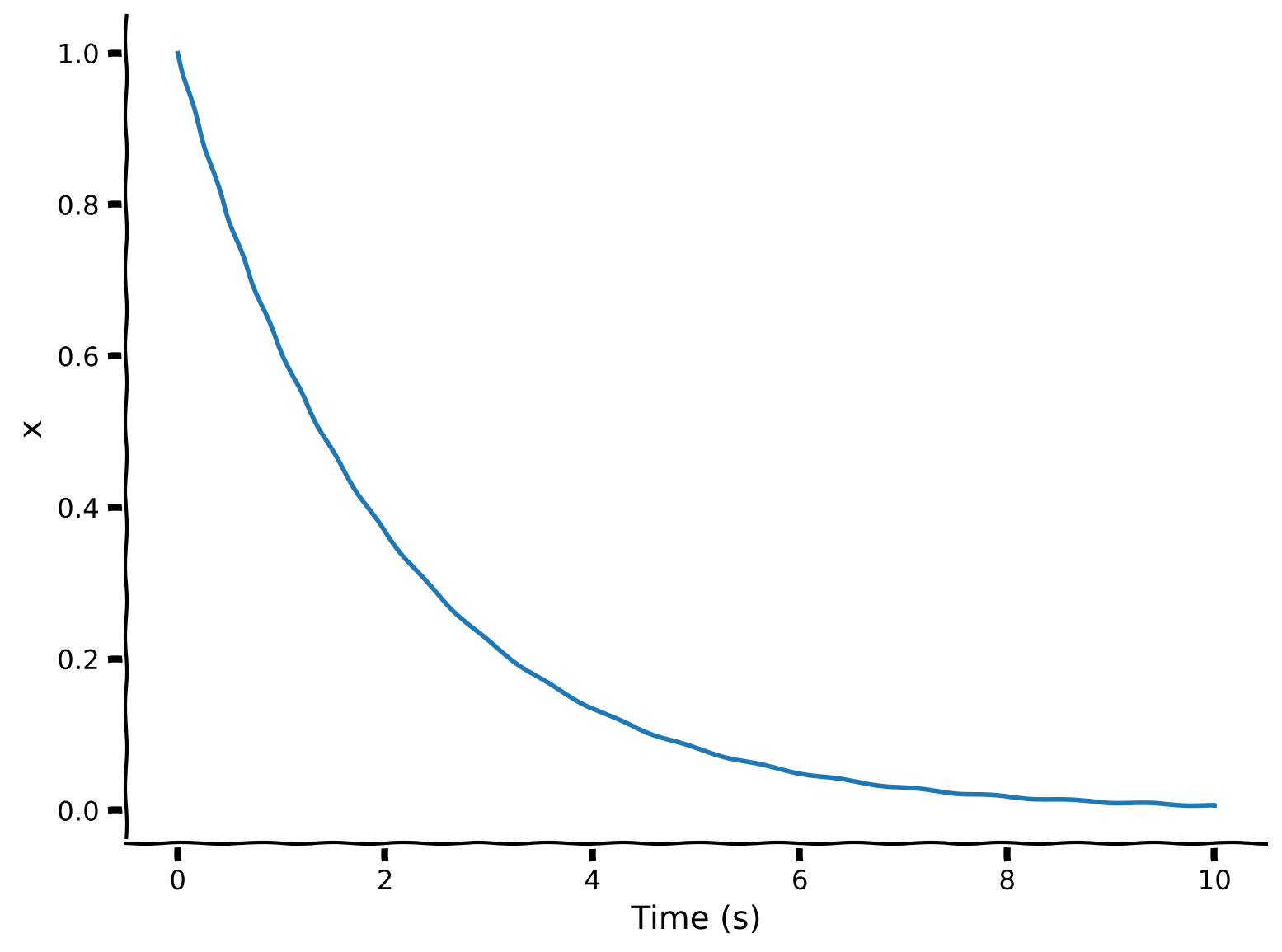
In this exercise, we will complete a function, integrate_exponential, to compute the solution of the differential equation \(\dot{x} = a x\) using forward Euler integration. We will then plot this solution over time.
def integrate_exponential(a, x0, dt, T):
  """Compute solution of the differential equation xdot=a*x with
  initial condition x0 for a duration T. Use time step dt for numerical
  solution.

  Args:
    a (scalar): parameter of xdot (xdot=a*x)
    x0 (scalar): initial condition (x at time 0)
    dt (scalar): timestep of the simulation
    T (scalar): total duration of the simulation

  Returns:
    ndarray, ndarray: `x` for all simulation steps and the time `t` at each step
  """

  # Initialize variables
  t = np.arange(0, T, dt)
  x = np.zeros_like(t, dtype=complex)
  x[0] = x0 # This is x at time t_0

  # Step through system and integrate in time
  for k in range(1, len(t)):

    ###################################################################
    ## Fill out the following then remove
    raise NotImplementedError("Student exercise: need to implement simulation")
    ###################################################################

    # for each point in time, compute xdot from x[k-1]
    xdot = ...

    # Update x based on x[k-1] and xdot
    x[k] = ...

  return x, t


# Choose parameters
a = -0.5    # parameter in f(x)
T = 10      # total Time duration
dt = 0.001  # timestep of our simulation
x0 = 1.     # initial condition of x at time 0

# Use Euler's method
x, t = integrate_exponential(a, x0, dt, T)

# Visualize
plt.plot(t, x.real)
plt.xlabel('Time (s)')
plt.ylabel('x')
plt.show()
Example output:
Submit your feedback#
Show code cell source
# @title Submit your feedback
content_review(f"{feedback_prefix}_Forward_Euler_Integration_Exercise")
Interactive Demo 1: Forward Euler Integration#
What happens when you change \(a\)? Try values where \(a<0\) and \(a>0\).
The \(dt\) is the step size of the forward Euler integration. Try \(a = -1.5\) and increase \(dt\). What happens to the numerical solution when you increase \(dt\)?
Make sure you execute this cell to enable the widget!
Show code cell source
# @markdown Make sure you execute this cell to enable the widget!

T = 10  # total Time duration
x0 = 1.  # initial condition of x at time 0

@widgets.interact(
    a=widgets.FloatSlider(value=-0.5, min=-2.5, max=1.5, step=0.25,
                          description="α", readout_format='.2f'),
    dt=widgets.FloatSlider(value=0.001, min=0.001, max=1.0, step=0.001,
                           description="dt", readout_format='.3f')
    )

def plot_euler_integration(a, dt):
  # Have to do this clunky word around to show small values in slider accurately
  # (from https://github.com/jupyter-widgets/ipywidgets/issues/259)

  x, t = integrate_exponential(a, x0, dt, T)
  plt.plot(t, x.real)  # integrate_exponential returns complex
  plt.xlabel('Time (s)')
  plt.ylabel('x')
  plt.show()
Submit your feedback#
Show code cell source
# @title Submit your feedback
content_review(f"{feedback_prefix}_What_models_Video")
Section 2: Oscillatory Dynamics#
Estimated timing to here from start of tutorial: 20 min
Video 2: Oscillatory Solutions#
Submit your feedback#
Show code cell source
# @title Submit your feedback
content_review(f"{feedback_prefix}_Forward_Euler_Integration_Interactive_Demo_Discussion")
We will now explore what happens when \(a\) is a complex number and has a non-zero imaginary component.
Interactive Demo 2: Oscillatory Dynamics#
Referred to as exercise 1B in video
In the following demo, you can change the real part and imaginary part of \(a\) (so a = real + imaginary i)
What values of \(a\) produce dynamics that both oscillate and grow?
What value of \(a\) is needed to produce a stable oscillation of 0.5 Hertz (cycles/time units)?
Make sure you execute this cell to enable the widget!
Show code cell source
# @markdown Make sure you execute this cell to enable the widget!

# parameters
T = 5  # total Time duration
dt = 0.0001  # timestep of our simulation
x0 = 1.  # initial condition of x at time 0

@widgets.interact
def plot_euler_integration(real=(-2, 2, .2), imaginary=(-4, 7, .1)):

  a = complex(real, imaginary)
  x, t = integrate_exponential(a, x0, dt, T)
  plt.plot(t, x.real)  # integrate exponential returns complex
  plt.grid(True)
  plt.xlabel('Time (s)')
  plt.ylabel('x')
  plt.show()
Submit your feedback#
Show code cell source
# @title Submit your feedback
content_review(f"{feedback_prefix}_Oscillatory_Dynamics_Interactive_Demo_Discussion")
Section 3: Deterministic Linear Dynamics in Two Dimensions#
Estimated timing to here from start of tutorial: 33 min
Video 3: Multi-Dimensional Dynamics#
Submit your feedback#
Show code cell source
# @title Submit your feedback
content_review(f"{feedback_prefix}_MultiDimensional_Dynamics_Video")
This video serves as an introduction to two-dimensional, deterministic dynamical systems written as a vector-matrix equation. It covers stream plots and how to connect phase portraits with the eigenvalues and eigenvectors of the transition matrix A.
Click here for text recap of relevant part of video
Adding one additional variable (or dimension) adds more variety of behaviors. Additional variables are useful in modeling the dynamics of more complex systems with richer behaviors, such as systems of multiple neurons. We can write such a system using two linear ordinary differential equations:
So far, this system consists of two variables (e.g. neurons) in isolation. To make things interesting, we can add interaction terms:
We can write the two equations that describe our system as one (vector-valued) linear ordinary differential equation:
For two-dimensional systems, \(\mathbf{x}\) is a vector with 2 elements (\(x_1\) and \(x_2\)) and \(\mathbf{A}\) is a \(2 \times 2\) matrix with \(\mathbf{A}=\bigg[\begin{array} & a_{11} & a_{12} \\ a_{21} & a_{22} \end{array} \bigg]\).
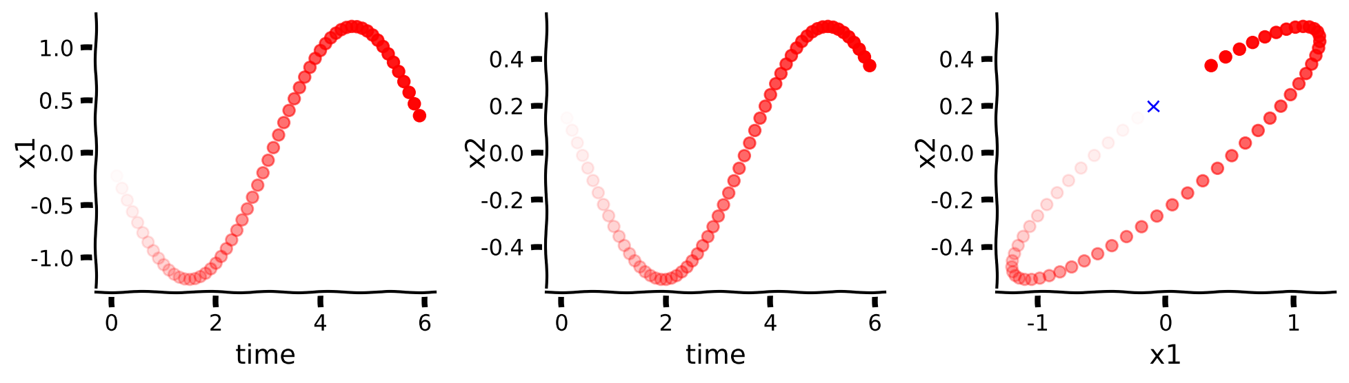
Coding Exercise 3: Sample trajectories in 2 dimensions#
Referred to in video as step 1 and 2 of exercise 1C
We want to simulate some trajectories of a given system and plot how 𝑥1 and 𝑥2 evolve in time. We will begin with this example system:
We will use an integrator from scipy, so we won’t have to solve the system ourselves. We have a helper function, plot_trajectory, that plots these trajectories given a system function. In this exercise, we will write the system function for a linear system with two variables.
def system(t, x, a00, a01, a10, a11):
  '''
  Compute the derivative of the state x at time t for a linear
  differential equation with A matrix [[a00, a01], [a10, a11]].

  Args:
    t (float): time
    x (ndarray): state variable
    a00, a01, a10, a11 (float): parameters of the system

  Returns:
    ndarray: derivative xdot of state variable x at time t
  '''
  #################################################
  ## TODO for students: Compute xdot1 and xdot2 ##
  ## Fill out the following then remove
  raise NotImplementedError("Student exercise: say what they should have done")
  #################################################

  # compute x1dot and x2dot
  x1dot = ...
  x2dot = ...

  return np.array([x1dot, x2dot])


# Set parameters
T = 6 # total time duration
dt = 0.1 # timestep of our simulation
A = np.array([[2, -5],
              [1, -2]])
x0 = [-0.1, 0.2]

# Simulate and plot trajectories
plot_trajectory(system, [A[0, 0], A[0, 1], A[1, 0], A[1, 1]], x0, dt=dt, T=T)
Example output:
Submit your feedback#
Show code cell source
# @title Submit your feedback
content_review(f"{feedback_prefix}_Sample_trajectories_in_2_dimensions_Exercise")
Interactive Demo 3A: Varying A#
We will now use the function we created in the last exercise to plot trajectories with different options for A. What kinds of qualitatively different dynamics do you observe?
Hint: Keep an eye on the x-axis and y-axis!
Make sure you execute this cell to enable the widget!
Show code cell source
# @markdown Make sure you execute this cell to enable the widget!

# parameters
T = 6  # total Time duration
dt = 0.1  # timestep of our simulation
x0 = np.asarray([-0.1, 0.2])  # initial condition of x at time 0

A_option_1 = [[2, -5],[1, -2]]
A_option_2 = [[3,4], [1, 2]]
A_option_3 = [[-1, -1], [0, -0.25]]
A_option_4 = [[3, -2],[2, -2]]

@widgets.interact
def plot_euler_integration(A=widgets.Dropdown(options=[A_option_1,
                                                       A_option_2,
                                                       A_option_3,
                                                       A_option_4,
                                                       None],
                                              value=A_option_1)):
  if A:
    plot_trajectory(system, [A[0][0],A[0][1],A[1][0],A[1][1]], x0, dt=dt, T=T)
Submit your feedback#
Show code cell source
# @title Submit your feedback
content_review(f"{feedback_prefix}_Varying_A_Interactive_Demo_Discussion")
Interactive Demo 3B: Varying Initial Conditions#
We will now vary the initial conditions for a given \(\mathbf{A}\):
What kinds of qualitatively different dynamics do you observe? Hint: Keep an eye on the x-axis and y-axis!
Make sure you execute this cell to enable the widget!
Show code cell source
# @markdown Make sure you execute this cell to enable the widget!

# parameters
T = 6  # total Time duration
dt = 0.1  # timestep of our simulation
x0 = np.asarray([-0.1, 0.2])  # initial condition of x at time 0
A = [[2, -5],[1, -2]]

x0_option_1 = [-.1, 0.2]
x0_option_2 = [10, 10]
x0_option_3 = [-4, 3]

@widgets.interact
def plot_euler_integration(x0 = widgets.Dropdown(options=[x0_option_1,
                                                          x0_option_2,
                                                          x0_option_3,
                                                          None],
                                                 value=x0_option_1)):
  if x0:
    plot_trajectory(system, [A[0][0], A[0][1], A[1][0], A[1][1]], x0, dt=dt, T=T)
Submit your feedback#
Show code cell source
# @title Submit your feedback
content_review(f"{feedback_prefix}_Varying_Initial_Conditions_Interactive_Demo_Discussion")
Section 4: Stream Plots#
Estimated timing to here from start of tutorial: 45 min
It’s a bit tedious to plot trajectories one initial condition at a time!
Fortunately, to get an overview of how a grid of initial conditions affect trajectories of a system, we can use a stream plot.
We can think of a initial condition \({\bf x}_0=(x_{1_0},x_{2_0})\) as coordinates for a position in a space. For a 2x2 matrix \(\bf A\), a stream plot computes at each position \(\bf x\) a small arrow that indicates \(\bf Ax\) and then connects the small arrows to form stream lines. Remember from the beginning of this tutorial that \(\dot {\bf x} = \bf Ax\) is the rate of change of \(\bf x\). So the stream lines indicate how a system changes. If you are interested in a particular initial condition \({\bf x}_0\), just find the corresponding position in the stream plot. The stream line that goes through that point in the stream plot indicates \({\bf x}(t)\).
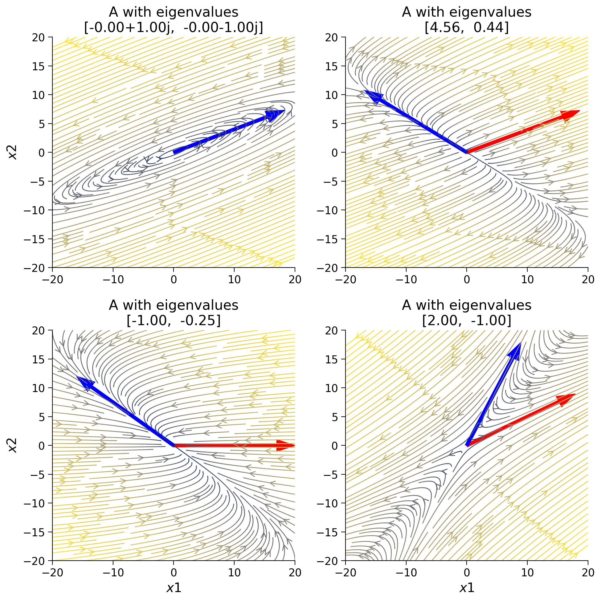
Think! 4: Interpreting Eigenvalues and Eigenvectors#
Using some helper functions, we show the stream plots for each option of A that you examined in the earlier interactive demo. We included the eigenvectors of \(\bf A\) as a red line (1st eigenvalue) and a blue line (2nd eigenvalue) in the stream plots.
What is special about the direction in which the principal eigenvector points? And how does the stability of the system relate to the corresponding eigenvalues? (Hint: Remember from your introduction to linear algebra that, for matrices with real eigenvalues, the eigenvectors indicate the lines on which \(\bf Ax\) is parallel to \(\bf x\) and real eigenvalues indicate the factor by which \(\bf Ax\) is stretched or shrunk compared to \(\bf x\).)
Execute this cell to see stream plots
Show code cell source
# @markdown Execute this cell to see stream plots

A_option_1 = np.array([[2, -5], [1, -2]])
A_option_2 = np.array([[3,4], [1, 2]])
A_option_3 = np.array([[-1, -1], [0, -0.25]])
A_option_4 = np.array([[3, -2], [2, -2]])

A_options = [A_option_1, A_option_2, A_option_3, A_option_4]
plot_specific_example_stream_plots(A_options)
Submit your feedback#
Show code cell source
# @title Submit your feedback
content_review(f"{feedback_prefix}_Interpreting_Eigenvalues_and_Eigenvectors_Discussion")
Summary#
Estimated timing of tutorial: 1 hour
In this tutorial, we learned:
How to simulate the trajectory of a dynamical system specified by a differential equation \(\dot{x} = f(x)\) using a forward Euler integration scheme.
The behavior of a one-dimensional linear dynamical system \(\dot{x} = a x\) is determined by \(a\), which may be a complex valued number. Knowing \(a\), we know about the stability and oscillatory dynamics of the system.
The dynamics of high-dimensional linear dynamical systems \(\dot{\mathbf{x}} = \mathbf{A} \mathbf{x}\) can be understood using the same intuitions, where we can summarize the behavior of the trajectories using the eigenvalues and eigenvectors of \(\mathbf{A}\).