Tutorial 1: Neural Rate Models

Tutorial 1: Neural Rate Models#

Week 2, Day 4: Dynamic Networks

By Neuromatch Academy

Content creators: Qinglong Gu, Songtin Li, Arvind Kumar, John Murray, Julijana Gjorgjieva

Content reviewers: Maryam Vaziri-Pashkam, Ella Batty, Lorenzo Fontolan, Richard Gao, Spiros Chavlis, Michael Waskom, Siddharth Suresh

Production editors: Gagana B, Spiros Chavlis

Tutorial Objectives#

Estimated timing of tutorial: 1 hour, 25 minutes

The brain is a complex system, not because it is composed of a large number of diverse types of neurons, but mainly because of how neurons are connected to each other. The brain is indeed a network of highly specialized neuronal networks.

The activity of a neural network constantly evolves in time. For this reason, neurons can be modeled as dynamical systems. The dynamical system approach is only one of the many modeling approaches that computational neuroscientists have developed (other points of view include information processing, statistical models, etc.).

How the dynamics of neuronal networks affect the representation and processing of information in the brain is an open question. However, signatures of altered brain dynamics present in many brain diseases (e.g., in epilepsy or Parkinson’s disease) tell us that it is crucial to study network activity dynamics if we want to understand the brain.

In this tutorial, we will simulate and study one of the simplest models of biological neuronal networks. Instead of modeling and simulating individual excitatory neurons (e.g., LIF models that you implemented yesterday), we will treat them as a single homogeneous population and approximate their dynamics using a single one-dimensional equation describing the evolution of their average spiking rate in time.

In this tutorial, we will learn how to build a firing rate model of a single population of excitatory neurons.

Steps:

Write the equation for the firing rate dynamics of a 1D excitatory population.
Visualize the response of the population as a function of parameters such as threshold level and gain, using the frequency-current (F-I) curve.
Numerically simulate the dynamics of the excitatory population and find the fixed points of the system.

Setup#

Install and import feedback gadget#

# Imports
import matplotlib.pyplot as plt
import numpy as np
import scipy.optimize as opt  # root-finding algorithm

Figure Settings#

Plotting Functions#

Section 1: Neuronal network dynamics#

Video 1: Dynamic networks#

This video covers how to model a network with a single population of neurons and introduces neural rate-based models. It overviews feedforward networks and defines the F-I (firing rate vs. input) curve.

Submit your feedback#

Section 1.1: Dynamics of a single excitatory population#

Click here for text recap of relevant part of video

Individual neurons respond by spiking. When we average the spikes of neurons in a population, we can define the average firing activity of the population. In this model, we are interested in how the population-averaged firing varies as a function of time and network parameters. Mathematically, we can describe the firing rate dynamic of a feed-forward network as:

(309)#\[\begin{equation} \tau \frac{dr}{dt} = -r + F(I_{\text{ext}}) \quad\qquad (1) \end{equation}\]

\(r(t)\) represents the average firing rate of the excitatory population at time \(t\), \(\tau\) controls the timescale of the evolution of the average firing rate, \(I_{\text{ext}}\) represents the external input, and the transfer function \(F(\cdot)\) (which can be related to f-I curve of individual neurons described in the next sections) represents the population activation function in response to all received inputs.

To start building the model, please execute the cell below to initialize the simulation parameters.

Execute this cell to set default parameters for a single excitatory population model

{'tau': 1.0, 'a': 1.2, 'theta': 2.8, 'w': 0.0, 'I_ext': 0.0, 'T': 20.0, 'dt': 0.1, 'r_init': 0.2, 'range_t': array([ 0. ,  0.1,  0.2,  0.3,  0.4,  0.5,  0.6,  0.7,  0.8,  0.9,  1. ,
        1.1,  1.2,  1.3,  1.4,  1.5,  1.6,  1.7,  1.8,  1.9,  2. ,  2.1,
        2.2,  2.3,  2.4,  2.5,  2.6,  2.7,  2.8,  2.9,  3. ,  3.1,  3.2,
        3.3,  3.4,  3.5,  3.6,  3.7,  3.8,  3.9,  4. ,  4.1,  4.2,  4.3,
        4.4,  4.5,  4.6,  4.7,  4.8,  4.9,  5. ,  5.1,  5.2,  5.3,  5.4,
        5.5,  5.6,  5.7,  5.8,  5.9,  6. ,  6.1,  6.2,  6.3,  6.4,  6.5,
        6.6,  6.7,  6.8,  6.9,  7. ,  7.1,  7.2,  7.3,  7.4,  7.5,  7.6,
        7.7,  7.8,  7.9,  8. ,  8.1,  8.2,  8.3,  8.4,  8.5,  8.6,  8.7,
        8.8,  8.9,  9. ,  9.1,  9.2,  9.3,  9.4,  9.5,  9.6,  9.7,  9.8,
        9.9, 10. , 10.1, 10.2, 10.3, 10.4, 10.5, 10.6, 10.7, 10.8, 10.9,
       11. , 11.1, 11.2, 11.3, 11.4, 11.5, 11.6, 11.7, 11.8, 11.9, 12. ,
       12.1, 12.2, 12.3, 12.4, 12.5, 12.6, 12.7, 12.8, 12.9, 13. , 13.1,
       13.2, 13.3, 13.4, 13.5, 13.6, 13.7, 13.8, 13.9, 14. , 14.1, 14.2,
       14.3, 14.4, 14.5, 14.6, 14.7, 14.8, 14.9, 15. , 15.1, 15.2, 15.3,
       15.4, 15.5, 15.6, 15.7, 15.8, 15.9, 16. , 16.1, 16.2, 16.3, 16.4,
       16.5, 16.6, 16.7, 16.8, 16.9, 17. , 17.1, 17.2, 17.3, 17.4, 17.5,
       17.6, 17.7, 17.8, 17.9, 18. , 18.1, 18.2, 18.3, 18.4, 18.5, 18.6,
       18.7, 18.8, 18.9, 19. , 19.1, 19.2, 19.3, 19.4, 19.5, 19.6, 19.7,
       19.8, 19.9])}

You can now use:

pars = default_pars_single() to get all the parameters.
pars = default_pars_single(T=T_sim, dt=time_step) to set new simulation time and time step
To update an existing parameter dictionary, use pars['New_para'] = value

Because pars is a dictionary, it can be passed to a function that requires individual parameters as arguments using my_func(**pars) syntax.

Section 1.2: F-I curves#

Estimated timing to here from start of tutorial: 17 min

Click here for text recap of relevant part of video

In electrophysiology, a neuron is often characterized by its spike rate output in response to input currents. This is often called the F-I curve, denoting the output spike frequency (F) in response to different injected currents (I). We estimated this for an LIF neuron in yesterday’s tutorial.

The transfer function \(F(\cdot)\) in Equation \(1\) represents the gain of the population as a function of the total input. The gain is often modeled as a sigmoidal function, i.e., more input drive leads to a nonlinear increase in the population firing rate. The output firing rate will eventually saturate for high input values.

A sigmoidal \(F(\cdot)\) is parameterized by its gain \(a\) and threshold \(\theta\).

\[ F(x;a,\theta) = \frac{1}{1+\text{e}^{-a(x-\theta)}} - \frac{1}{1+\text{e}^{a\theta}} \quad(2)\]

The argument \(x\) represents the input to the population. Note that the second term is chosen so that \(F(0;a,\theta)=0\).

Many other transfer functions (generally monotonic) can be also used. Examples are the rectified linear function \(ReLU(x)\) or the hyperbolic tangent \(tanh(x)\).

Coding Exercise 1.2: Implement F-I curve#

Let’s first investigate the activation functions before simulating the dynamics of the entire population.

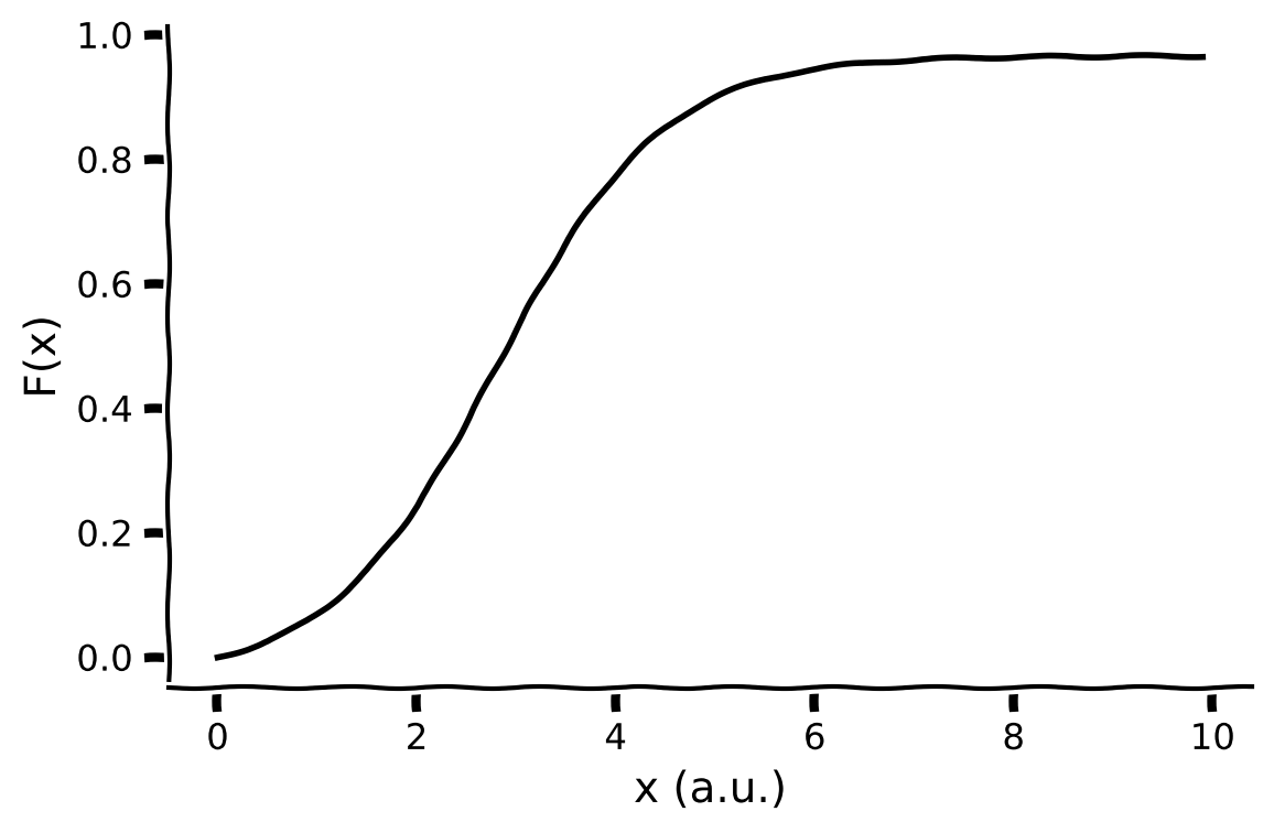
In this exercise, you will implement a sigmoidal F-I curve or transfer function \(F(x)\), with gain \(a\) and threshold level \(\theta\) as parameters:

(310)#\[\begin{equation} F(x;a,\theta) = \frac{1}{1+\text{e}^{-a(x-\theta)}} - \frac{1}{1+\text{e}^{a\theta}} \end{equation}\]

def F(x, a, theta):
  """
  Population activation function.

  Args:
    x (float): the population input
    a (float): the gain of the function
    theta (float): the threshold of the function

  Returns:
    float: the population activation response F(x) for input x
  """
  #################################################
  ## TODO for students: compute f = F(x) ##
  # Fill out function and remove
  raise NotImplementedError("Student exercise: implement the f-I function")
  #################################################

  # Define the sigmoidal transfer function f = F(x)
  f = ...

  return f


# Set parameters
pars = default_pars_single()  # get default parameters
x = np.arange(0, 10, .1)      # set the range of input

# Compute transfer function
f = F(x, pars['a'], pars['theta'])

# Visualize
plot_fI(x, f)

Click for solution

Example output:

Submit your feedback#

Interactive Demo 1.2 : Parameter exploration of F-I curve#

Here’s an interactive demo that shows how the F-I curve changes for different values of the gain and threshold parameters.

How does the gain parameter (\(a\)) affect the F-I curve?
How does the threshold parameter (\(\theta\)) affect the F-I curve?

Make sure you execute this cell to enable the widget!

<Figure size 800x600 with 0 Axes>

Click for solution

Submit your feedback#

Section 1.3: Simulation scheme of E dynamics#

Estimated timing to here from start of tutorial: 27 min

Because \(F(\cdot)\) is a nonlinear function, the exact solution of our differential equation of population activity can not be determined via analytical methods. As we have seen before, we can use numerical methods, specifically the Euler method, to find the solution (that is, simulate the population activity).

Execute this cell to enable the single population rate model simulator: simulate_single

Help on function simulate_single in module __main__:

simulate_single(pars)
    Simulate an excitatory population of neurons
    
    Args:
      pars   : Parameter dictionary
    
    Returns:
      rE     : Activity of excitatory population (array)
    
    Example:
      pars = default_pars_single()
      r = simulate_single(pars)

Interactive Demo 1.3: Parameter Exploration of single population dynamics#

Explore these dynamics of the population activity in this interactive demo.

How does \(r_{\text{sim}}(t)\) change with different \(I_{\text{ext}}\) values?
How does it change with different \(\tau\) values?

Note that, \(r_{\rm ana}(t)\) denotes the analytical solution - you will learn how this is computed in the next section.

#

Make sure you execute this cell to enable the widget!

Click for solution

Submit your feedback#

Think! 1.3: Finite activities#

Above, we have numerically solved a system driven by a positive input. Yet, \(r_E(t)\) either decays to zero or reaches a fixed non-zero value.

Why doesn’t the solution of the system “explode” in a finite time? In other words, what guarantees that \(r_E\)(t) stays finite?
Which parameter would you change in order to increase the maximum value of the response?

Click for solution

Submit your feedback#

Section 2: Fixed points of the single population system#

Estimated timing to here from start of tutorial: 45 min

Section 2.1: Finding fixed points#

Video 2: Fixed point#

Submit your feedback#

This video introduces recurrent networks and how to derive their fixed points. It also introduces vector fields and phase planes in one dimension.

Click here for text recap of video

We can now extend our feed-forward network to a recurrent network, governed by the equation:

(311)#\[\begin{align} \tau \frac{dr}{dt} &= -r + F(w\cdot r + I_{\text{ext}}) \quad\qquad (3) \end{align}\]

where as before, \(r(t)\) represents the average firing rate of the excitatory population at time \(t\), \(\tau\) controls the timescale of the evolution of the average firing rate, \(I_{\text{ext}}\) represents the external input, and the transfer function \(F(\cdot)\) (which can be related to f-I curve of individual neurons described in the next sections) represents the population activation function in response to all received inputs. Now we also have \(w\) which denotes the strength (synaptic weight) of the recurrent input to the population.

As you varied the two parameters in the last Interactive Demo, you noticed that, while at first the system output quickly changes, with time, it reaches its maximum/minimum value and does not change anymore. The value eventually reached by the system is called the steady state of the system, or the fixed point. Essentially, in the steady states the derivative with respect to time of the activity (\(r\)) is zero, i.e. \(\displaystyle \frac{dr}{dt}=0\).

We can find that the steady state of the Equation. (1) by setting \(\displaystyle{\frac{dr}{dt}=0}\) and solve for \(r\):

(312)#\[\begin{equation} -r_{\text{steady}} + F(w\cdot r_{\text{steady}} + I_{\text{ext}};a,\theta) = 0 \qquad (4) \end{equation}\]

When it exists, the solution of Equation. (4) defines a fixed point of the dynamical system in Equation (3). Note that if \(F(x)\) is nonlinear, it is not always possible to find an analytical solution, but the solution can be found via numerical simulations, as we will do later.

From the Interactive Demo, one could also notice that the value of \(\tau\) influences how quickly the activity will converge to the steady state from its initial value.

In the specific case of \(w=0\), we can also analytically compute the solution of Equation (1) (i.e., the thick blue dashed line) and deduce the role of \(\tau\) in determining the convergence to the fixed point:

(313)#\[\begin{equation} \displaystyle{r(t) = \big{[}F(I_{\text{ext}};a,\theta) -r(t=0)\big{]} (1-\text{e}^{-\frac{t}{\tau}})} + r(t=0) \end{equation}\]

We can now numerically calculate the fixed point with a root finding algorithm.

Coding Exercise 2.1.1: Visualization of the fixed points#

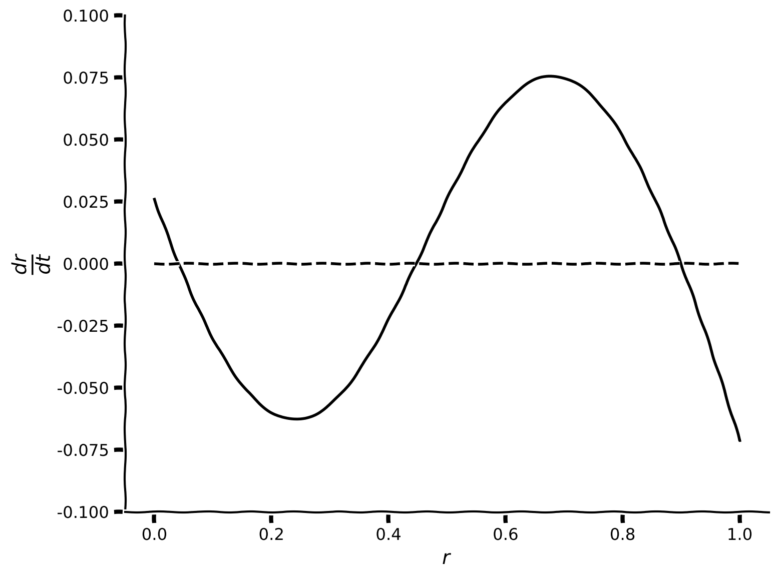
When it is not possible to find the solution for Equation (3) analytically, a graphical approach can be taken. To that end, it is useful to plot \(\displaystyle{\frac{dr}{dt}}\) as a function of \(r\). The values of \(r\) for which the plotted function crosses zero on the y axis correspond to fixed points.

Here, let us, for example, set \(w=5.0\) and \(I^{\text{ext}}=0.5\). From Equation (3), you can obtain

(314)#\[\begin{equation} \frac{dr}{dt} = [-r + F(w\cdot r + I^{\text{ext}})]\,/\,\tau \end{equation}\]

Then, plot the \(dr/dt\) as a function of \(r\), and check for the presence of fixed points.

def compute_drdt(r, I_ext, w, a, theta, tau, **other_pars):
  """Given parameters, compute dr/dt as a function of r.

  Args:
    r (1D array) : Average firing rate of the excitatory population
    I_ext, w, a, theta, tau (numbers): Simulation parameters to use
    other_pars : Other simulation parameters are unused by this function

  Returns
    drdt function for each value of r
  """
  #########################################################################
  # TODO compute drdt and disable the error
  raise NotImplementedError("Finish the compute_drdt function")
  #########################################################################

  # Calculate drdt
  drdt = ...

  return drdt


# Define a vector of r values and the simulation parameters
r = np.linspace(0, 1, 1000)
pars = default_pars_single(I_ext=0.5, w=5)

# Compute dr/dt
drdt = compute_drdt(r, **pars)

# Visualize
plot_dr_r(r, drdt)

Click for solution

Example output:

Submit your feedback#

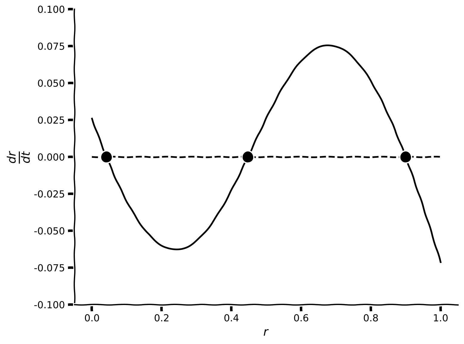
Coding Exercise 2.1.2: Numerical calculation of fixed points#

We will now find the fixed points numerically. To do so, we need to specify initial values (\(r_{\text{guess}}\)) for the root-finding algorithm to start from. From the line \(\displaystyle{\frac{dr}{dt}}\) plotted above in the last exercise, initial values can be chosen as a set of values close to where the line crosses zero on the y axis (real fixed point).

The next cell defines three helper functions that we will use:

my_fp_single(r_guess, **pars) uses a root-finding algorithm to locate a fixed point near a given initial value
check_fp_single(x_fp, **pars) verifies that the values of \(r_{\rm fp}\) for which \(\displaystyle{\frac{dr}{dt}} = 0\) are the true fixed points
my_fp_finder(r_guess_vector, **pars) accepts an array of initial values and finds the same number of fixed points, using the above two functions

Execute this cell to enable the fixed point functions

Help on function my_fp_finder in module __main__:

my_fp_finder(pars, r_guess_vector, mytol=0.0001)
    Calculate the fixed point(s) through drE/dt=0
    
    Args:
      pars    : Parameter dictionary
      r_guess_vector  : Initial values used for scipy.optimize function
      mytol   : tolerance for checking fixed point, default as 10^{-4}
    
    Returns:
      x_fps   : values of fixed points

# Set parameters
r = np.linspace(0, 1, 1000)
pars = default_pars_single(I_ext=0.5, w=5)

# Compute dr/dt
drdt = compute_drdt(r, **pars)

#############################################################################
# TODO for students:
# Define initial values close to the intersections of drdt and y=0
# (How many initial values? Hint: How many times do the two lines intersect?)
# Calculate the fixed point with these initial values and plot them
raise NotImplementedError('student_exercise: find fixed points numerically')
#############################################################################

# Initial guesses for fixed points
r_guess_vector = [...]

# Find fixed point numerically
x_fps = my_fp_finder(pars, r_guess_vector)

# Visualize
plot_dr_r(r, drdt, x_fps)

Click for solution

Example output:

Submit your feedback#

Interactive Demo 2.1: fixed points as a function of recurrent and external inputs.#

You can now explore how the previous plot changes when the recurrent coupling \(w\) and the external input \(I_{\text{ext}}\) take different values. How does the number of fixed points change?

Make sure you execute this cell to enable the widget!

Click for solution

Submit your feedback#

Section 2.2: Relationship between trajectories & fixed points#

Let’s examine the relationship between the population activity over time and the fixed points.

Here, let us first set \(w=5.0\) and \(I_{\text{ext}}=0.5\), and investigate the dynamics of \(r(t)\) starting with different initial values \(r(0) \equiv r_{\text{init}}\).

Execute to visualize dr/dt

Interactive Demo 2.2: dynamics as a function of the initial value#

Let’s now set \(r_{\rm init}\) to a value of your choice in this demo. How does the solution change? What do you observe? How does that relate to the previous plot of \(\frac{dr}{dt}\)?

Make sure you execute this cell to enable the widget!

Click for solution

Submit your feedback#

We will plot the trajectories of \(r(t)\) with \(r_{\text{init}} = 0.0, 0.1, 0.2,..., 0.9\).

Execute this cell to see the trajectories!

We have three fixed points but only two steady states showing up - what’s happening?

It turns out that the stability of the fixed points matters. If a fixed point is stable, a trajectory starting near that fixed point will stay close to that fixed point and converge to it (the steady state will equal the fixed point). If a fixed point is unstable, any trajectories starting close to it will diverge and go towards stable fixed points. In fact, the only way for a trajectory to reach a stable state at an unstable fixed point is if the initial value exactly equals the value of the fixed point.

Think! 2.2: Stable vs unstable fixed points#

Which of the fixed points for the model we’ve been examining in this section are stable vs unstable?

Execute to print fixed point values

Click for solution

Submit your feedback#

We can simulate the trajectory if we start at the unstable fixed point: you can see that it remains at that fixed point (the red line below).

Execute to visualize trajectory starting at unstable fixed point

See Bonus Section 1 to cover how to determine the stability of fixed points in a quantitative way.

Think! 2: Inhibitory populations#

Throughout the tutorial, we have assumed \(w> 0 \), i.e., we considered a single population of excitatory neurons. What do you think will be the behavior of a population of inhibitory neurons, i.e., where \(w> 0\) is replaced by \(w< 0\)?

Click for solution

Submit your feedback#

Summary#

Estimated timing of tutorial: 1 hour, 25 minutes

In this tutorial, we have investigated the dynamics of a rate-based single population of neurons.

We learned about:

The effect of the input parameters and the time constant of the network on the dynamics of the population.
How to find the fixed point(s) of the system.

We build on these concepts in the bonus material - check it out if you have time. You will learn:

How to determine the stability of a fixed point by linearizing the system.
How to add realistic inputs to our model.

Bonus#

Bonus Section 1: Stability analysis via linearization of the dynamics#

Video 3: Stability of fixed points#

Submit your feedback#

Here we will dive into the math of how to figure out the stability of a fixed point.

Just like in our equation for the feedforward network, a generic linear system \(\frac{dx}{dt} = \lambda (x - b)\), has a fixed point for \(x=b\). The analytical solution of such a system can be found to be:

(315)#\[\begin{equation} x(t) = b + \big{(} x(0) - b \big{)} \text{e}^{\lambda t}. \end{equation}\]

Now consider a small perturbation of the activity around the fixed point: \(x(0) = b + \epsilon\), where \(|\epsilon| \ll 1\). Will the perturbation \(\epsilon(t)\) grow with time or will it decay to the fixed point? The evolution of the perturbation with time can be written, using the analytical solution for \(x(t)\), as:

(316)#\[\begin{equation} \epsilon (t) = x(t) - b = \epsilon \text{e}^{\lambda t} \end{equation}\]

if \(\lambda < 0\), \(\epsilon(t)\) decays to zero, \(x(t)\) will still converge to \(b\) and the fixed point is “stable”.
if \(\lambda > 0\), \(\epsilon(t)\) grows with time, \(x(t)\) will leave the fixed point \(b\) exponentially, and the fixed point is, therefore, “unstable” .

Similar to what we did in the linear system above, in order to determine the stability of a fixed point \(r^{*}\) of the excitatory population dynamics, we perturb Equation (1) around \(r^{*}\) by \(\epsilon\), i.e. \(r = r^{*} + \epsilon\). We can plug in Equation (1) and obtain the equation determining the time evolution of the perturbation \(\epsilon(t)\):

(317)#\[\begin{equation} \tau \frac{d\epsilon}{dt} \approx -\epsilon + w F'(w\cdot r^{*} + I_{\text{ext}};a,\theta) \epsilon \end{equation}\]

where \(F'(\cdot)\) is the derivative of the transfer function \(F(\cdot)\). We can rewrite the above equation as:

(318)#\[\begin{equation} \frac{d\epsilon}{dt} \approx \frac{\epsilon}{\tau }[-1 + w F'(w\cdot r^* + I_{\text{ext}};a,\theta)] \end{equation}\]

That is, as in the linear system above, the value of

(319)#\[\begin{equation} \lambda = [-1+ wF'(w\cdot r^* + I_{\text{ext}};a,\theta)]/\tau \qquad (4) \end{equation}\]

determines whether the perturbation will grow or decay to zero, i.e., \(\lambda\) defines the stability of the fixed point. This value is called the eigenvalue of the dynamical system.

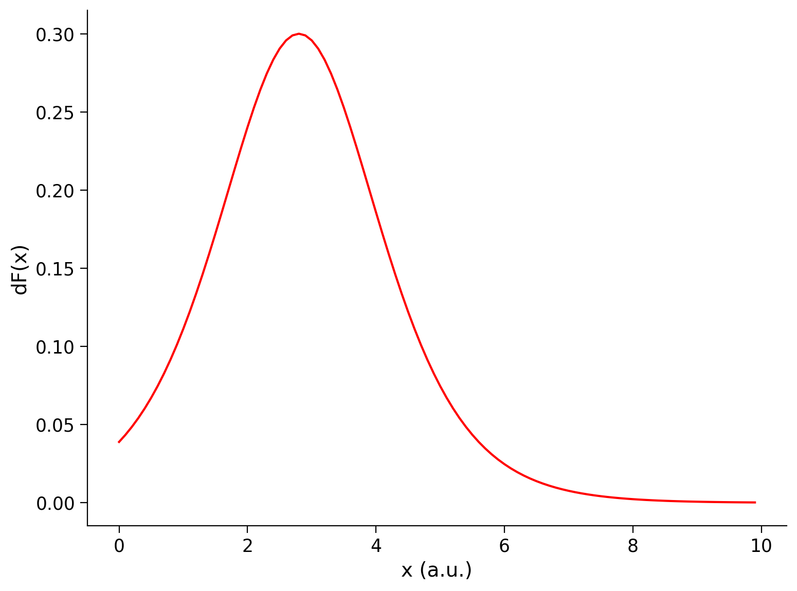
The derivative of the sigmoid transfer function is:

(320)#\[\begin{align} \frac{dF}{dx} & = \frac{d}{dx} (1+\exp\{-a(x-\theta)\})^{-1} \\ & = a\exp\{-a(x-\theta)\} (1+\exp\{-a(x-\theta)\})^{-2}. \qquad (5) \end{align}\]

We provide a helper function dF which computes this derivative.

Execute this cell to enable helper function dF and visualize derivative

../../../_images/1b363041fb5fb61a3a23a6585599118b0e19eb9b8b18f2f2c7ab09a8cc143b51.png

Bonus Coding Exercise 1: Compute eigenvalues#

As discussed above, for the case with \(w=5.0\) and \(I_{\text{ext}}=0.5\), the system displays three fixed points. However, when we simulated the dynamics and varied the initial conditions \(r_{\rm init}\), we could only obtain two steady states. In this exercise, we will now check the stability of each of the three fixed points by calculating the corresponding eigenvalues with the function eig_single. Check the sign of each eigenvalue (i.e., stability of each fixed point). How many of the fixed points are stable?

Note that the expression of the eigenvalue at fixed point \(r^*\):

(321)#\[\begin{equation} \lambda = [-1+ wF'(w\cdot r^* + I_{\text{ext}};a,\theta)]/\tau \end{equation}\]

def eig_single(fp, tau, a, theta, w, I_ext, **other_pars):
  """
  Args:
    fp   : fixed point r_fp
    tau, a, theta, w, I_ext : Simulation parameters

  Returns:
    eig : eigenvalue of the linearized system
  """
  #####################################################################
  ## TODO for students: compute eigenvalue and disable the error
  raise NotImplementedError("Student exercise: compute the eigenvalue")
  ######################################################################
  # Compute the eigenvalue
  eig = ...

  return eig


# Find the eigenvalues for all fixed points
pars = default_pars_single(w=5, I_ext=.5)
r_guess_vector = [0, .4, .9]
x_fp = my_fp_finder(pars, r_guess_vector)


for fp in x_fp:
  eig_fp = eig_single(fp, **pars)
  print(f'Fixed point1 at {fp:.3f} with Eigenvalue={eig_fp:.3f}')

SAMPLE OUTPUT

Fixed point1 at 0.042 with Eigenvalue=-0.583
Fixed point2 at 0.447 with Eigenvalue=0.498
Fixed point3 at 0.900 with Eigenvalue=-0.626

Click for solution

Submit your feedback#

We can see that the first and third fixed points are stable (negative eigenvalues) and the second is unstable (positive eigenvalue) - as we expected!

Bonus Section 2: Noisy input drives the transition between two stable states#

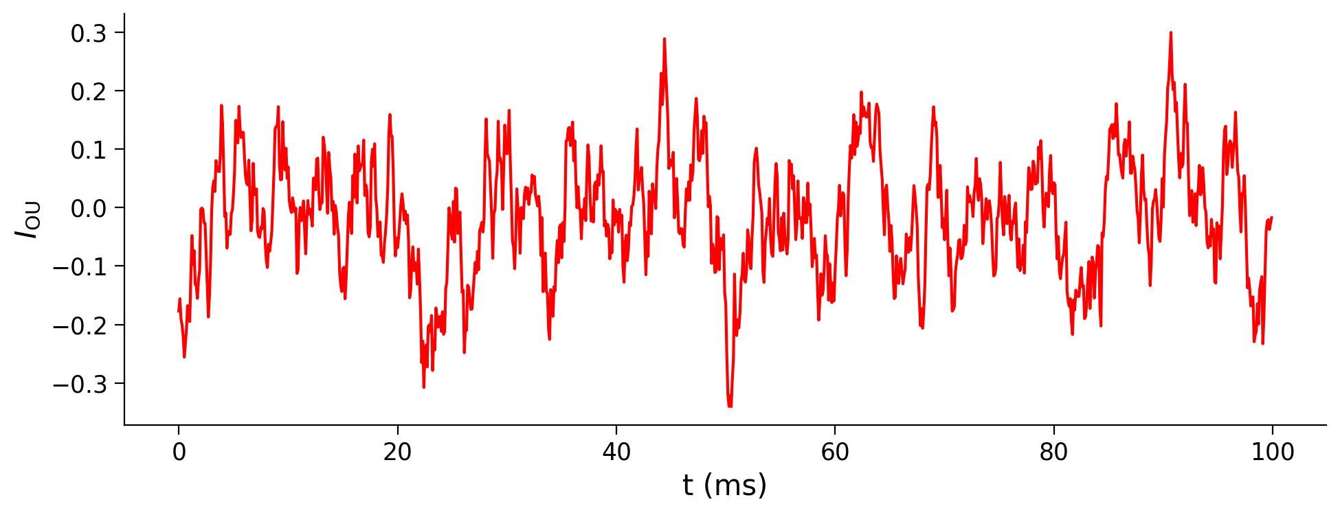
As discussed in several previous tutorials, the Ornstein-Uhlenbeck (OU) process is usually used to generate a noisy input into the neuron. The OU input \(\eta(t)\) follows:

(322)#\[\begin{equation} \tau_\eta \frac{d}{dt}\eta(t) = -\eta (t) + \sigma_\eta\sqrt{2\tau_\eta}\xi(t) \end{equation}\]

Execute the following function my_OU(pars, sig, myseed=False) to generate an OU process.

Execute to get helper function my_OU and visualize OU process

../../../_images/66b978e811c0940f37034c9bc560d47da9e0ae20094dab32517922434af3941c.png

In the presence of two or more fixed points, noisy inputs can drive a transition between the fixed points! Here, we stimulate an E population for 1,000 ms applying OU inputs.

Execute this cell to simulate E population with OU inputs

You can see that the population activity is changing between fixed points (it goes up and down)!

Tutorial 1: Neural Rate Models

Contents

Tutorial 1: Neural Rate Models#

Tutorial Objectives#

Setup#

Install and import feedback gadget#

Figure Settings#

Plotting Functions#

Section 1: Neuronal network dynamics#

Video 1: Dynamic networks#

Submit your feedback#

Section 1.1: Dynamics of a single excitatory population#

Section 1.2: F-I curves#

Coding Exercise 1.2: Implement F-I curve#

Submit your feedback#

Interactive Demo 1.2 : Parameter exploration of F-I curve#

Submit your feedback#

Section 1.3: Simulation scheme of E dynamics#

Interactive Demo 1.3: Parameter Exploration of single population dynamics#

#

Submit your feedback#

Think! 1.3: Finite activities#

Submit your feedback#

Section 2: Fixed points of the single population system#

Section 2.1: Finding fixed points#

Video 2: Fixed point#

Submit your feedback#

Coding Exercise 2.1.1: Visualization of the fixed points#

Submit your feedback#

Coding Exercise 2.1.2: Numerical calculation of fixed points#

Submit your feedback#

Interactive Demo 2.1: fixed points as a function of recurrent and external inputs.#

Submit your feedback#

Section 2.2: Relationship between trajectories & fixed points#

Interactive Demo 2.2: dynamics as a function of the initial value#

Submit your feedback#

Think! 2.2: Stable vs unstable fixed points#

Submit your feedback#

Think! 2: Inhibitory populations#

Submit your feedback#

Summary#

Bonus#

Bonus Section 1: Stability analysis via linearization of the dynamics#

Video 3: Stability of fixed points#

Submit your feedback#

Bonus Coding Exercise 1: Compute eigenvalues#

Submit your feedback#

Bonus Section 2: Noisy input drives the transition between two stable states#