Tutorial 1: The Leaky Integrate-and-Fire (LIF) Neuron Model

Tutorial 1: The Leaky Integrate-and-Fire (LIF) Neuron Model#

Week 2, Day 3: Biological Neuron Models

By Neuromatch Academy

Content creators: Qinglong Gu, Songtin Li, John Murray, Richard Naud, Arvind Kumar

Content reviewers: Maryam Vaziri-Pashkam, Ella Batty, Lorenzo Fontolan, Richard Gao, Matthew Krause, Spiros Chavlis, Michael Waskom, Ethan Cheng

Production editors: Gagana B, Spiros Chavlis

Tutorial Objectives#

Estimated timing of tutorial: 1 hour, 10 min

This is Tutorial 1 of a series on implementing realistic neuron models. In this tutorial, we will build up a leaky integrate-and-fire (LIF) neuron model and study its dynamics in response to various types of inputs. In particular, we are going to write a few lines of code to:

simulate the LIF neuron model
drive the LIF neuron with external inputs, such as direct currents, Gaussian white noise, and Poisson spike trains, etc.
study how different inputs affect the LIF neuron’s output (firing rate and spike time irregularity)

Here, we will especially emphasize identifying conditions (input statistics) under which a neuron can spike at low firing rates and in an irregular manner. The reason for focusing on this is that in most cases, neocortical neurons spike in an irregular manner.

Setup#

Install and import feedback gadget#

# Imports
import numpy as np
import matplotlib.pyplot as plt

Figure Settings#

Plotting Functions#

Show code cell source Hide code cell source

# @title Plotting Functions

def plot_volt_trace(pars, v, sp):
  """
  Plot trajetory of membrane potential for a single neuron

  Expects:
  pars   : parameter dictionary
  v      : volt trajetory
  sp     : spike train

  Returns:
  figure of the membrane potential trajetory for a single neuron
  """

  V_th = pars['V_th']
  dt, range_t = pars['dt'], pars['range_t']
  if sp.size:
    sp_num = (sp / dt).astype(int) - 1
    v[sp_num] += 20  # draw nicer spikes

  plt.plot(pars['range_t'], v, 'b')
  plt.axhline(V_th, 0, 1, color='k', ls='--')
  plt.xlabel('Time (ms)')
  plt.ylabel('V (mV)')
  plt.legend(['Membrane\npotential', r'Threshold V$_{\mathrm{th}}$'],
             loc=[1.05, 0.75])
  plt.ylim([-80, -40])
  plt.show()


def plot_GWN(pars, I_GWN):
  """
  Args:
    pars  : parameter dictionary
    I_GWN : Gaussian white noise input

  Returns:
    figure of the gaussian white noise input
  """

  plt.figure(figsize=(12, 4))
  plt.subplot(121)
  plt.plot(pars['range_t'][::3], I_GWN[::3], 'b')
  plt.xlabel('Time (ms)')
  plt.ylabel(r'$I_{GWN}$ (pA)')
  plt.subplot(122)
  plot_volt_trace(pars, v, sp)
  plt.tight_layout()
  plt.show()


def my_hists(isi1, isi2, cv1, cv2, sigma1, sigma2):
  """
  Args:
    isi1 : vector with inter-spike intervals
    isi2 : vector with inter-spike intervals
    cv1  : coefficient of variation for isi1
    cv2  : coefficient of variation for isi2

  Returns:
    figure with two histograms, isi1, isi2

  """
  plt.figure(figsize=(11, 4))
  my_bins = np.linspace(10, 30, 20)
  plt.subplot(121)
  plt.hist(isi1, bins=my_bins, color='b', alpha=0.5)
  plt.xlabel('ISI (ms)')
  plt.ylabel('count')
  plt.title(r'$\sigma_{GWN}=$%.1f, CV$_{\mathrm{isi}}$=%.3f' % (sigma1, cv1))

  plt.subplot(122)
  plt.hist(isi2, bins=my_bins, color='b', alpha=0.5)
  plt.xlabel('ISI (ms)')
  plt.ylabel('count')
  plt.title(r'$\sigma_{GWN}=$%.1f, CV$_{\mathrm{isi}}$=%.3f' % (sigma2, cv2))
  plt.tight_layout()
  plt.show()

Section 1: The Leaky Integrate-and-Fire (LIF) model#

Video 1: Reduced Neuron Models#

Submit your feedback#

This video introduces the reduction of a biological neuron to a simple leaky-integrate-fire (LIF) neuron model.

Click here for text recap of video

Now, it’s your turn to implement one of the simplest mathematical model of a neuron: the leaky integrate-and-fire (LIF) model. The basic idea of LIF neuron was proposed in 1907 by Louis Édouard Lapicque, long before we understood the electrophysiology of a neuron (see a translation of Lapicque’s paper ). More details of the model can be found in the book Theoretical neuroscience by Peter Dayan and Laurence F. Abbott.

The subthreshold membrane potential dynamics of a LIF neuron is described by

(282)#\[\begin{eqnarray} C_m\frac{dV}{dt} = -g_L(V-E_L) + I,\quad (1) \end{eqnarray}\]

where \(C_m\) is the membrane capacitance, \(V\) is the membrane potential, \(g_L\) is the leak conductance (\(g_L = 1/R\), the inverse of the leak resistance \(R\) mentioned in previous tutorials), \(E_L\) is the resting potential, and \(I\) is the external input current.

Dividing both sides of the above equation by \(g_L\) gives

(283)#\[\begin{align} \tau_m\frac{dV}{dt} = -(V-E_L) + \frac{I}{g_L}\,,\quad (2) \end{align}\]

where the \(\tau_m\) is membrane time constant and is defined as \(\tau_m=C_m/g_L\).

Note that dividing capacitance by conductance gives units of time!

Below, we will use Eqn.(2) to simulate LIF neuron dynamics.

If \(I\) is sufficiently strong such that \(V\) reaches a certain threshold value \(V_{\rm th}\), \(V\) is reset to a reset potential \(V_{\rm reset}< V_{\rm th}\), and voltage is clamped to \(V_{\rm reset}\) for \(\tau_{\rm ref}\) ms, mimicking the refractoriness of the neuron during an action potential:

(284)#\[\begin{eqnarray} \mathrm{if}\quad V(t_{\text{sp}})\geq V_{\rm th}&:& V(t)=V_{\rm reset} \text{ for } t\in(t_{\text{sp}}, t_{\text{sp}} + \tau_{\text{ref}}] \end{eqnarray}\]

where \(t_{\rm sp}\) is the spike time when \(V(t)\) just exceeded \(V_{\rm th}\).

(Note: in the lecture slides, \(\theta\) corresponds to the threshold voltage \(V_{th}\), and \(\Delta\) corresponds to the refractory time \(\tau_{\rm ref}\).)

Note that you have seen the LIF model before if you looked at the pre-reqs Python or Calculus days!

The LIF model captures the facts that a neuron:

performs spatial and temporal integration of synaptic inputs
generates a spike when the voltage reaches a certain threshold
goes refractory during the action potential
has a leaky membrane

The LIF model assumes that the spatial and temporal integration of inputs is linear. Also, membrane potential dynamics close to the spike threshold are much slower in LIF neurons than in real neurons.

Coding Exercise 1: Python code to simulate the LIF neuron#

We now write Python code to calculate our equation for the LIF neuron and simulate the LIF neuron dynamics. We will use the Euler method, which you saw in the linear systems case yesterday to numerically integrate this equation:

(285)#\[\begin{equation} \tau_m\frac{dV}{dt} = -(V-E_L) + \frac{I}{g_L}\, \end{equation}\]

where \(V\) is the membrane potential, \(g_L\) is the leak conductance, \(E_L\) is the resting potential, \(I\) is the external input current, and \(\tau_m\) is membrane time constant.

The cell below initializes a dictionary that stores parameters of the LIF neuron model and the simulation scheme. You can use pars=default_pars(T=simulation_time, dt=time_step) to get the parameters. Note that, simulation_time and time_step have the unit ms. In addition, you can add the value to a new parameter by pars['New_param'] = value.

Execute this code to initialize the default parameters

{'V_th': -55.0, 'V_reset': -75.0, 'tau_m': 10.0, 'g_L': 10.0, 'V_init': -75.0, 'E_L': -75.0, 'tref': 2.0, 'T': 400.0, 'dt': 0.1, 'range_t': array([0.000e+00, 1.000e-01, 2.000e-01, ..., 3.997e+02, 3.998e+02,
       3.999e+02])}

Complete the function below to simulate the LIF neuron when receiving external current inputs. You can use v, sp = run_LIF(pars, Iinj) to get the membrane potential (v) and spike train (sp) given the dictionary pars and input current Iinj.

def run_LIF(pars, Iinj, stop=False):
  """
  Simulate the LIF dynamics with external input current

  Args:
    pars       : parameter dictionary
    Iinj       : input current [pA]. The injected current here can be a value
                 or an array
    stop       : boolean. If True, use a current pulse

  Returns:
    rec_v      : membrane potential
    rec_sp     : spike times
  """

  # Set parameters
  V_th, V_reset = pars['V_th'], pars['V_reset']
  tau_m, g_L = pars['tau_m'], pars['g_L']
  V_init, E_L = pars['V_init'], pars['E_L']
  dt, range_t = pars['dt'], pars['range_t']
  Lt = range_t.size
  tref = pars['tref']

  # Initialize voltage
  v = np.zeros(Lt)
  v[0] = V_init

  # Set current time course
  Iinj = Iinj * np.ones(Lt)

  # If current pulse, set beginning and end to 0
  if stop:
    Iinj[:int(len(Iinj) / 2) - 1000] = 0
    Iinj[int(len(Iinj) / 2) + 1000:] = 0

  # Loop over time
  rec_spikes = []  # record spike times
  tr = 0.  # the count for refractory duration

  for it in range(Lt - 1):

    if tr > 0:  # check if in refractory period
      v[it] = V_reset  # set voltage to reset
      tr = tr - 1 # reduce running counter of refractory period

    elif v[it] >= V_th:  # if voltage over threshold
      rec_spikes.append(it)  # record spike event
      v[it] = V_reset  # reset voltage
      tr = tref / dt  # set refractory time

    ########################################################################
    ## TODO for students: compute the membrane potential v, spike train sp #
    # Fill out function and remove
    raise NotImplementedError('Student Exercise: calculate the dv/dt and the update step!')
    ########################################################################

    # Calculate the increment of the membrane potential
    dv = ...

    # Update the membrane potential
    v[it + 1] = ...

  # Get spike times in ms
  rec_spikes = np.array(rec_spikes) * dt

  return v, rec_spikes


# Get parameters
pars = default_pars(T=500)

# Simulate LIF model
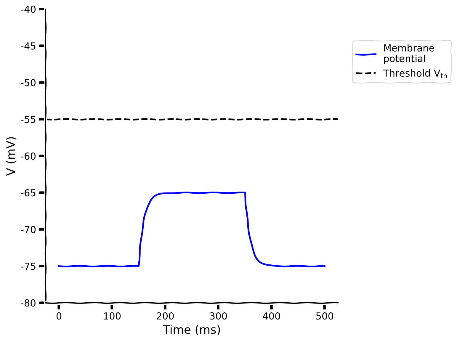
v, sp = run_LIF(pars, Iinj=100, stop=True)

# Visualize
plot_volt_trace(pars, v, sp)

Click for solution

Example output:

Submit your feedback#

Section 2: Response of an LIF model to different types of input currents#

Estimated timing to here from start of tutorial: 20 min

In the following section, we will learn how to inject direct current and white noise to study the response of an LIF neuron.

Video 2: Response of the LIF neuron to different inputs#

Submit your feedback#

Section 2.1: Direct current (DC)#

Estimated timing to here from start of tutorial: 30 min

Interactive Demo 2.1: Parameter exploration of DC input amplitude#

Here’s an interactive demo that shows how the LIF neuron behavior changes for DC input (constant current) with different amplitudes. We plot the membrane potential of an LIF neuron. You may notice that the neuron generates a spike. But this is just a cosmetic spike only for illustration purposes. In an LIF neuron, we only need to keep track of times when the neuron hits the threshold so the postsynaptic neurons can be informed of the spike.

How much DC is needed to reach the threshold (rheobase current)? How does the membrane time constant affect the frequency of the neuron?

Make sure you execute this cell to enable the widget!

Click for solution

Submit your feedback#

Section 2.2: Gaussian white noise (GWN) current#

Estimated timing to here from start of tutorial: 38 min

Given the noisy nature of neuronal activity in vivo, neurons usually receive complex, time-varying inputs.

To mimic this, we will now investigate the neuronal response when the LIF neuron receives Gaussian white noise \(\xi(t)\) with mean 0 (\(\mu = 0\)) and some standard deviation \(\sigma\).

Note that the GWN has zero mean, that is, it describes only the fluctuations of the input received by a neuron. We can thus modify our definition of GWN to have a nonzero mean value \(\mu\) that equals the DC input, since this is the average input into the cell. The cell below defines the modified gaussian white noise currents with nonzero mean \(\mu\).

Interactive Demo 2.2: LIF neuron Explorer for noisy input#

The mean of the Gaussian white noise (GWN) is the amplitude of DC. Indeed, when \(\sigma = 0\), GWN is just a DC.

So the question arises how does \(\sigma\) of the GWN affect the spiking behavior of the neuron. For instance we may want to know

how does the minimum input (i.e., \(\mu\)) needed to make a neuron spike change with increase in \(\sigma\)
how does the spike regularity change with increase in \(\sigma\)

To get an intuition about these questions you can use the following interactive demo that shows how the LIF neuron behavior changes for noisy input with different amplitudes (the mean \(\mu\)) and fluctuation sizes (\(\sigma\)). We use a helper function to generate this noisy input current: my_GWN(pars, mu, sig, myseed=False). Note that fixing the value of the random seed (e.g., myseed=2020) will allow you to obtain the same result every time you run this. We then use our run_LIF function to simulate the LIF model.

Execute to enable helper function my_GWN

Help on function my_GWN in module __main__:

my_GWN(pars, mu, sig, myseed=False)
    Function that generates Gaussian white noise input
    
    Args:
      pars       : parameter dictionary
      mu         : noise baseline (mean)
      sig        : noise amplitute (standard deviation)
      myseed     : random seed. int or boolean
                   the same seed will give the same
                   random number sequence
    
    Returns:
      I          : Gaussian white noise input

Make sure you execute this cell to enable the widget!

Click for solution

Submit your feedback#

Think! 2.2: Analyzing GWN Effects on Spiking#

As we increase the input average (\(\mu\)) or the input fluctuation (\(\sigma\)), the spike count changes. How much can we increase the spike count, and what might be the relationship between GWN mean/std or DC value and spike count?
We have seen above that when we inject DC, the neuron spikes in a regular manner (clock-like), and this regularity is reduced when GWN is injected. The question is, how irregular can we make the neurons spiking by changing the parameters of the GWN?

We will see the answers to these questions in the next section but discuss first!

Submit your feedback#

Section 3: Firing rate and spike time irregularity#

Estimated timing to here from start of tutorial: 48 min

When we plot the output firing rate as a function of GWN mean or DC value, it is called the input-output transfer function of the neuron (so simply F-I curve).

Spike regularity can be quantified as the coefficient of variation (CV) of the interspike interval (ISI):

(286)#\[\begin{equation} \text{CV}_{\text{ISI}} = \frac{std(\text{ISI})}{mean(\text{ISI})} \end{equation}\]

A Poisson train is an example of high irregularity, in which \(\textbf{CV}_{\textbf{ISI}} \textbf{= 1}\). And for a clocklike (regular) process we have \(\textbf{CV}_{\textbf{ISI}} \textbf{= 0}\) because of std(ISI)=0.

Interactive Demo 3A: F-I Explorer for different `sig_gwn`#

How does the F-I curve of the LIF neuron change as we increase the \(\sigma\) of the GWN? We can already expect that the F-I curve will be stochastic and the results will vary from one trial to another. But will there be any other change compared to the F-I curved measured using DC?

Here’s an interactive demo that shows how the F-I curve of a LIF neuron changes for different levels of fluctuation \(\sigma\).

Make sure you execute this cell to enable the widget!

Click for solution

Submit your feedback#

Coding Exercise 3: Compute \(CV_{ISI}\) values#

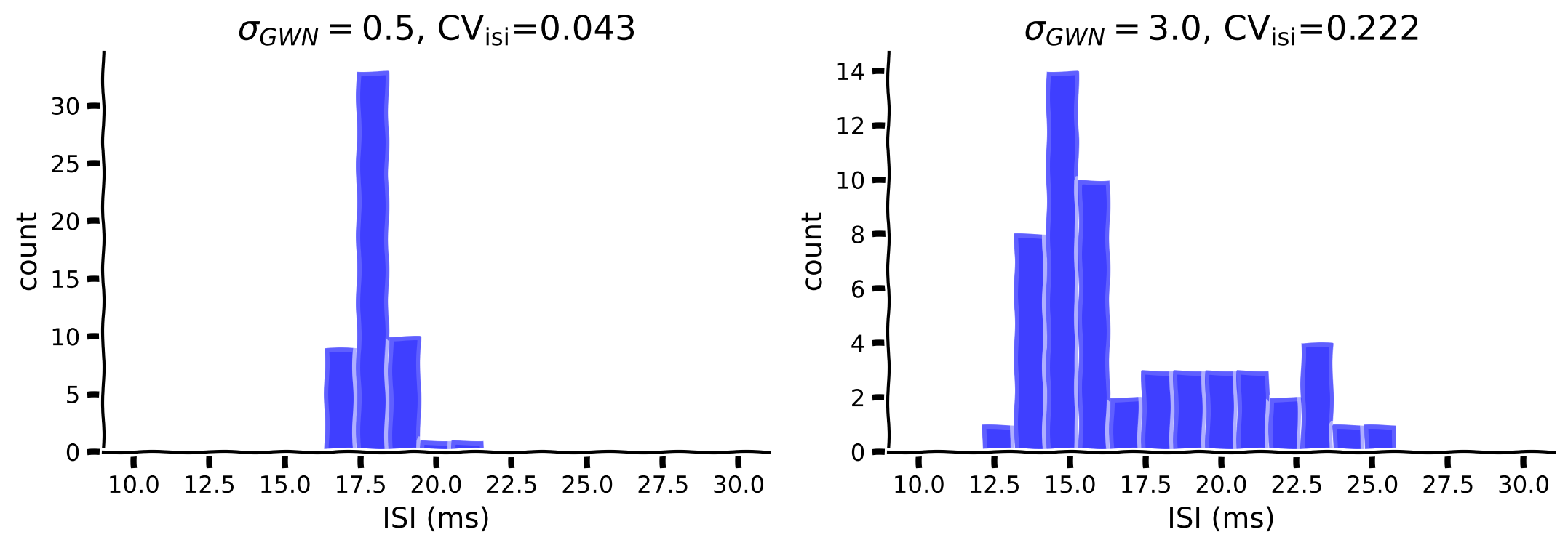
As shown above, the F-I curve becomes smoother while increasing the amplitude of the fluctuation (\(\sigma\)). In addition, the fluctuation can also change the irregularity of the spikes. Let’s investigate the effect of \(\mu=250\) with \(\sigma=0.5\) vs \(\sigma=3\).

Fill in the code below to compute ISI, then plot the histogram of the ISI and compute the \(CV_{ISI}\). Note that, you can use np.diff to calculate ISI.

def isi_cv_LIF(spike_times):
  """
  Calculates the interspike intervals (isi) and
  the coefficient of variation (cv) for a given spike_train

  Args:
    spike_times : (n, ) vector with the spike times (ndarray)

  Returns:
    isi         : (n-1,) vector with the inter-spike intervals (ms)
    cv          : coefficient of variation of isi (float)

  """
  ########################################################################
  ## TODO for students: compute the membrane potential v, spike train sp #
  # Fill out function and remove
  raise NotImplementedError('Student Exercise: calculate the isi and the cv!')
  ########################################################################
  if len(spike_times) >= 2:
    # Compute isi
    isi = ...
    # Compute cv
    cv = ...
  else:
    isi = np.nan
    cv = np.nan

  return isi, cv


# Set parameters
pars = default_pars(T=1000.)
mu_gwn = 250
sig_gwn1 = 0.5
sig_gwn2 = 3.0

# Run LIF model for sigma = 0.5
I_GWN1 = my_GWN(pars, mu=mu_gwn, sig=sig_gwn1, myseed=2020)
_, sp1 = run_LIF(pars, Iinj=I_GWN1)

# Run LIF model for sigma = 3
I_GWN2 = my_GWN(pars, mu=mu_gwn, sig=sig_gwn2, myseed=2020)
_, sp2 = run_LIF(pars, Iinj=I_GWN2)

# Compute ISIs/CV
isi1, cv1 = isi_cv_LIF(sp1)
isi2, cv2 = isi_cv_LIF(sp2)

# Visualize
my_hists(isi1, isi2, cv1, cv2, sig_gwn1, sig_gwn2)

Click for solution

Example output:

Submit your feedback#

Interactive Demo 3B: Spike irregularity explorer for different `sig_gwn`#

In the above illustration, we see that the CV of inter-spike-interval (ISI) distribution depends on \(\sigma\) of GWN. What about the mean of GWN, should that also affect the CV\(_{\rm ISI}\)? If yes, how? Does the efficacy of \(\sigma\) in increasing the CV\(_{\rm ISI}\) depend on \(\mu\)?

In the following interactive demo, you will examine how different levels of fluctuation \(\sigma\) affect the CVs for different average injected currents (\(\mu\)).

Does the standard deviation of the injected current affect the F-I curve in any qualitative manner?
Why does increasing the mean of GWN reduce the CV\(_{\rm ISI}\)?
If you plot spike count (or rate) vs. CV\(_{\rm ISI}\), should there be a relationship between the two? Try out yourself.

Make sure you execute this cell to enable the widget!

Click for solution

Submit your feedback#

Summary#

Estimated timing of tutorial: 1 hour, 10 min

Congratulations! You’ve just built a leaky integrate-and-fire (LIF) neuron model from scratch, and studied its dynamics in response to various types of inputs, having:

simulated the LIF neuron model
driven the LIF neuron with external inputs, such as direct current and Gaussian white noise
studied how different inputs affect the LIF neuron’s output (firing rate and spike time irregularity),

with a special focus on low rate and irregular firing regime to mimic real cortical neurons. The next tutorial will look at how spiking statistics may be influenced by a neuron’s input statistics.

If you have extra time, look at the bonus sections below to explore a different type of noise input and learn about extensions to integrate-and-fire models.

Bonus#

Bonus Section 1: Ornstein-Uhlenbeck Process#

When a neuron receives spiking input, the synaptic current is Shot Noise – which is a kind of colored noise and the spectrum of the noise determined by the synaptic kernel time constant. That is, a neuron is driven by colored noise and not GWN.

We can model colored noise using the Ornstein-Uhlenbeck process - filtered white noise.

We next study if the input current is temporally correlated and is modeled as an Ornstein-Uhlenbeck process \(\eta(t)\), i.e., low-pass filtered GWN with a time constant \(\tau_{\eta}\):

(287)#\[\begin{equation} \tau_\eta \frac{d}{dt}\eta(t) = \mu-\eta(t) + \sigma_\eta\sqrt{2\tau_\eta}\xi(t) \end{equation}\]

Hint: An OU process as defined above has

(288)#\[\begin{equation} \mathbb{E}[\eta(t)]=\mu \end{equation}\]

and autocovariance

(289)#\[\begin{equation} [\eta(t)\eta(t+\tau)]=\sigma_\eta^2e^{-|t-\tau|/\tau_\eta} \end{equation}\]

which can be used to check your code.

Execute this cell to get helper function my_OU

Help on function my_OU in module __main__:

my_OU(pars, mu, sig, myseed=False)
    Function that produces Ornstein-Uhlenbeck input
    
    Args:
      pars       : parameter dictionary
      sig        : noise amplitute
      myseed     : random seed. int or boolean
    
    Returns:
      I_ou       : Ornstein-Uhlenbeck input current

Bonus Interactive Demo 1: LIF Explorer with OU input#

In the following, we will check how a neuron responds to a noisy current that follows the statistics of an OU process.

How does the OU type input change neuron responsiveness?
What do you think will happen to the spike pattern and rate if you increased or decreased the time constant of the OU process?

Remember to enable the widget by running the cell!

Click for solution

Submit your feedback#

Bonus Section 2: Generalized Integrate-and-Fire models#

LIF model is not the only abstraction of real neurons. If you want to learn about more realistic types of neuronal models, watch the Bonus Video!

Tutorial 1: The Leaky Integrate-and-Fire (LIF) Neuron Model

Contents

Tutorial 1: The Leaky Integrate-and-Fire (LIF) Neuron Model#

Tutorial Objectives#

Setup#

Install and import feedback gadget#

Figure Settings#

Plotting Functions#

Section 1: The Leaky Integrate-and-Fire (LIF) model#

Video 1: Reduced Neuron Models#

Submit your feedback#

Coding Exercise 1: Python code to simulate the LIF neuron#

Submit your feedback#

Section 2: Response of an LIF model to different types of input currents#

Video 2: Response of the LIF neuron to different inputs#

Submit your feedback#

Section 2.1: Direct current (DC)#

Interactive Demo 2.1: Parameter exploration of DC input amplitude#

Submit your feedback#

Section 2.2: Gaussian white noise (GWN) current#

Interactive Demo 2.2: LIF neuron Explorer for noisy input#

Submit your feedback#

Think! 2.2: Analyzing GWN Effects on Spiking#

Submit your feedback#

Section 3: Firing rate and spike time irregularity#

Interactive Demo 3A: F-I Explorer for different `sig_gwn`#

Submit your feedback#

Coding Exercise 3: Compute \(CV_{ISI}\) values#

Submit your feedback#

Interactive Demo 3B: Spike irregularity explorer for different `sig_gwn`#

Submit your feedback#

Summary#

Bonus#

Bonus Section 1: Ornstein-Uhlenbeck Process#

Bonus Interactive Demo 1: LIF Explorer with OU input#

Submit your feedback#

Bonus Section 2: Generalized Integrate-and-Fire models#

Video 3 (Bonus): Extensions to Integrate-and-Fire models#

Submit your feedback#

Tutorial 1: The Leaky Integrate-and-Fire (LIF) Neuron Model

Contents

Tutorial 1: The Leaky Integrate-and-Fire (LIF) Neuron Model#

Tutorial Objectives#

Setup#

Install and import feedback gadget#

Figure Settings#

Plotting Functions#

Section 1: The Leaky Integrate-and-Fire (LIF) model#

Video 1: Reduced Neuron Models#

Submit your feedback#

Coding Exercise 1: Python code to simulate the LIF neuron#

Submit your feedback#

Section 2: Response of an LIF model to different types of input currents#

Video 2: Response of the LIF neuron to different inputs#

Submit your feedback#

Section 2.1: Direct current (DC)#

Interactive Demo 2.1: Parameter exploration of DC input amplitude#

Submit your feedback#

Section 2.2: Gaussian white noise (GWN) current#

Interactive Demo 2.2: LIF neuron Explorer for noisy input#

Submit your feedback#

Think! 2.2: Analyzing GWN Effects on Spiking#

Submit your feedback#

Section 3: Firing rate and spike time irregularity#

Interactive Demo 3A: F-I Explorer for different sig_gwn#

Submit your feedback#

Coding Exercise 3: Compute \(CV_{ISI}\) values#

Submit your feedback#

Interactive Demo 3B: Spike irregularity explorer for different sig_gwn#

Submit your feedback#

Summary#

Bonus#

Bonus Section 1: Ornstein-Uhlenbeck Process#

Bonus Interactive Demo 1: LIF Explorer with OU input#

Submit your feedback#

Bonus Section 2: Generalized Integrate-and-Fire models#

Video 3 (Bonus): Extensions to Integrate-and-Fire models#

Submit your feedback#

Interactive Demo 3A: F-I Explorer for different `sig_gwn`#

Interactive Demo 3B: Spike irregularity explorer for different `sig_gwn`#