Bonus Tutorial: Fitting to data

Bonus Tutorial: Fitting to data#

Week 3, Day 1: Bayesian Decisions

By Neuromatch Academy

Content creators: Vincent Valton, Konrad Kording

Content reviewers: Matt Krause, Jesse Livezey, Karolina Stosio, Saeed Salehi, Michael Waskom

Production editors: Gagana B, Spiros Chavlis

Note: This is bonus material, included from NMA 2020. It has not been substantially revised. This means that the notation and standards are slightly different and some of the references to other days in NMA are outdated. We include it here because it covers fitting Bayesian models to data, which may be of interest to many students.

Tutorial objectives#

In the first two tutorials, we learned about Bayesian models and decisions more intuitively, using demos. In this notebook, we will dive into using math and code to fit Bayesian models to data.

We’ll have a look at computing all the necessary steps to perform model inversion (estimate the model parameters such as \(p_{common}\) that generated data similar to that of a participant). We will describe all the steps of the generative model first, and in the last exercise we will use all these steps to estimate the parameter \(p_{common}\) of a single participant using simulated data.

The generative model will be a Bayesian model we saw in Tutorial 2: a mixture of Gaussian prior and a Gaussian likelihood.

Steps:

First, we’ll create the prior, likelihood, posterior, etc., in a form that will make it easier for us to visualize what is being computed and estimated at each step of the generative model:
1. Creating a mixture of Gaussian prior for multiple possible stimulus inputs
2. Generating the likelihood for multiple possible stimulus inputs
3. Estimating our posterior as a function of the stimulus input
4. Estimating a participant response given the posterior
Next, we’ll perform the model inversion/fitting: 5. Create a distribution for the input as a function of possible inputs 6. Marginalization 7. Generate some data using the generative model provided 8. Perform model inversion (model fitting) using the generated data and see if you recover the original parameters.

Setup#

Install and import feedback gadget#

# Imports
import numpy as np
import matplotlib.pyplot as plt
import matplotlib as mpl
from scipy.optimize import minimize

Figure Settings#

Plotting functions#

Show code cell source Hide code cell source

# @title Plotting functions

def plot_myarray(array, xlabel, ylabel, title):
  """ Plot an array with labels.

  Args :
    array (numpy array of floats)
    xlabel (string) - label of x-axis
    ylabel (string) - label of y-axis
    title  (string) - title of plot

  Returns:
    None
  """
  fig = plt.figure()
  ax = fig.add_subplot(111)
  colormap = ax.imshow(array, extent=[-10, 10, 8, -8])
  cbar = plt.colorbar(colormap, ax=ax)
  cbar.set_label('probability')
  ax.invert_yaxis()
  ax.set_xlabel(xlabel)
  ax.set_title(title)
  ax.set_ylabel(ylabel)
  ax.set_aspect('auto')
  return None


def plot_my_bayes_model(model) -> None:
  """Pretty-print a simple Bayes Model (ex 7), defined as a function:

  Args:
    - model: function that takes a single parameter value and returns
             the negative log-likelihood of the model, given that parameter
  Returns:
    None, draws plot
    """
  x = np.arange(-10,10,0.07)

  # Plot neg-LogLikelihood for different values of alpha
  alpha_tries = np.arange(0.01, 0.3, 0.01)
  nll = np.zeros_like(alpha_tries)
  for i_try in np.arange(alpha_tries.shape[0]):
    nll[i_try] = model(np.array([alpha_tries[i_try]]))

  plt.figure()
  plt.plot(alpha_tries, nll)
  plt.xlabel('p_independent value')
  plt.ylabel('negative log-likelihood')

  # Mark minima
  ix = np.argmin(nll)
  plt.scatter(alpha_tries[ix], nll[ix], c='r', s=144)

  #plt.axvline(alpha_tries[np.argmin(nll)])
  plt.title('Sample Output')
  plt.show()

  return None


def plot_simulated_behavior(true_stim, behaviour):
  fig = plt.figure(figsize=(7, 7))
  ax = fig.add_subplot(1,1,1)
  ax.set_facecolor('xkcd:light grey')
  plt.plot(true_stim, true_stim - behaviour, '-k', linewidth=2, label='data')
  plt.axvline(0, ls='dashed', color='grey')
  plt.axhline(0, ls='dashed', color='grey')
  plt.legend()
  plt.xlabel('Position of true visual stimulus (cm)')
  plt.ylabel('Participant deviation from true stimulus (cm)')
  plt.title('Participant behavior')
  plt.show()

  return None

Helper Functions#

Introduction#

Video 1: Intro#

Submit your feedback#

Here is a graphical representation of the generative model:

We present a stimulus \(x\) to participants.
The brain encodes this true stimulus \(x\) noisily (this is the brain’s representation of the true visual stimulus: \(p(\tilde x|x)\).
The brain then combines this brain-encoded stimulus (likelihood: \(p(\tilde x|x)\)) with prior information (the prior: \(p(x)\)) to make up the brain’s estimated position of the true visual stimulus, the posterior: \(p(x|\tilde x)\).
This brain’s estimated stimulus position: \(p(x|\tilde x)\), is then used to make a response: \(\hat x\), which is the participant’s noisy estimate of the stimulus position (the participant’s percept).

Typically the response \(\hat x\) also includes some motor noise (noise due to the hand/arm move not being 100% accurate), but we’ll ignore it in this tutorial and assume there is no motor noise.

We will use the same experimental setup as in tutorial 2 but with slightly different probabilities. This time, participants are told that they need to estimate the sound location of a puppet that is hidden behind a curtain. The participants are told to use auditory information and are also informed that the sound could come from 2 possible causes: a common cause (95% of the time, it comes from the puppet hidden behind the curtain at position 0) or an independent cause (5% of the time the sound comes from loud-speakers at more distant locations).

Section 1: Likelihood array#

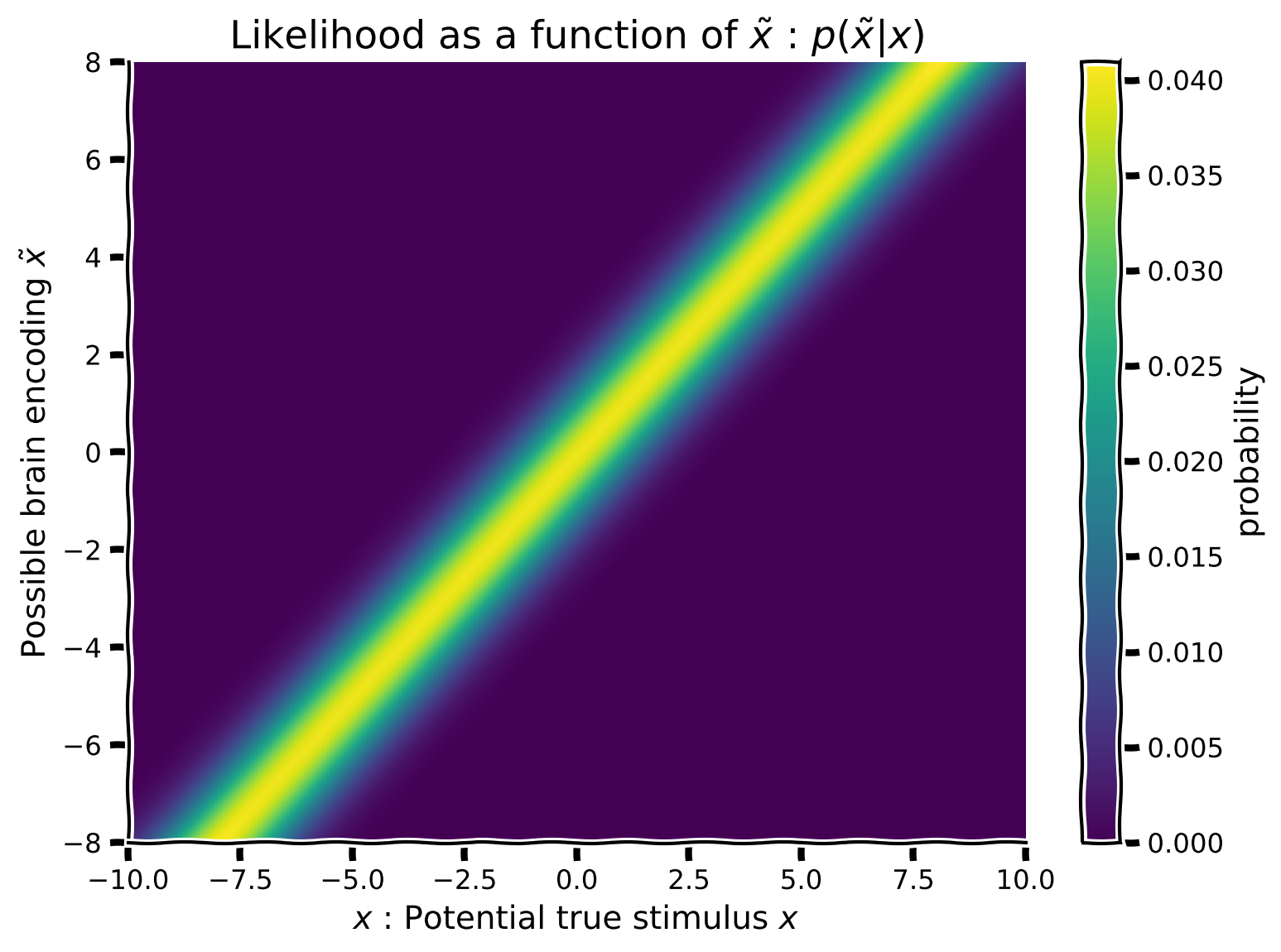
First, we want to create a likelihood, but for the sake of visualization (and to consider all possible brain encodings) we will create multiple likelihoods \(f(x)=p(\tilde x|x)\) (one for each potential encoded stimulus: \(\tilde x\)). We will then be able to visualize the likelihood as a function of hypothesized true stimulus positions: \(x\) on the x-axis and encoded position \(\tilde x\) on the y-axis.

Using the equation for the my_gaussian and the values in hypothetical_stim:

Create a Gaussian likelihood with mean varying from hypothetical_stim, keeping \(\sigma_{likelihood}\) constant at 1.
Each likelihood will have a different mean and thus a different row-likelihood of your 2D array, such that you end up with a likelihood array made up of 1,000 row-Gaussians with different means. (Hint: np.tile won’t work here. You may need a for-loop).
Plot the array using the function plot_myarray() already pre-written and commented-out in your script

Coding Exercise 1: Implement the auditory likelihood as a function of true stimulus position#

x = np.arange(-10, 10, 0.1)
hypothetical_stim = np.linspace(-8, 8, 1000)

def compute_likelihood_array(x_points, stim_array, sigma=1.):

  # initializing likelihood_array
  likelihood_array = np.zeros((len(stim_array), len(x_points)))
  # looping over stimulus array
  for i in range(len(stim_array)):
    ########################################################################
    ## Insert your code here to:
    ##      - Generate a likelihood array using `my_gaussian` function,
    ##        with std=1, and varying the mean using `stim_array` values.
    ## remove the raise below to test your function
    raise NotImplementedError("You need to complete the function!")
    ########################################################################
    likelihood_array[i, :] = ...

  return likelihood_array



likelihood_array = compute_likelihood_array(x, hypothetical_stim)
plot_myarray(likelihood_array,
             '$x$ : Potential true stimulus $x$',
             'Possible brain encoding $\~x$',
             'Likelihood as a function of $\~x$ : $p(\~x | x)$')

Click for solution

Example output:

Submit your feedback#

Section 2: Causal mixture of Gaussian prior#

Video 2: Prior array#

Submit your feedback#

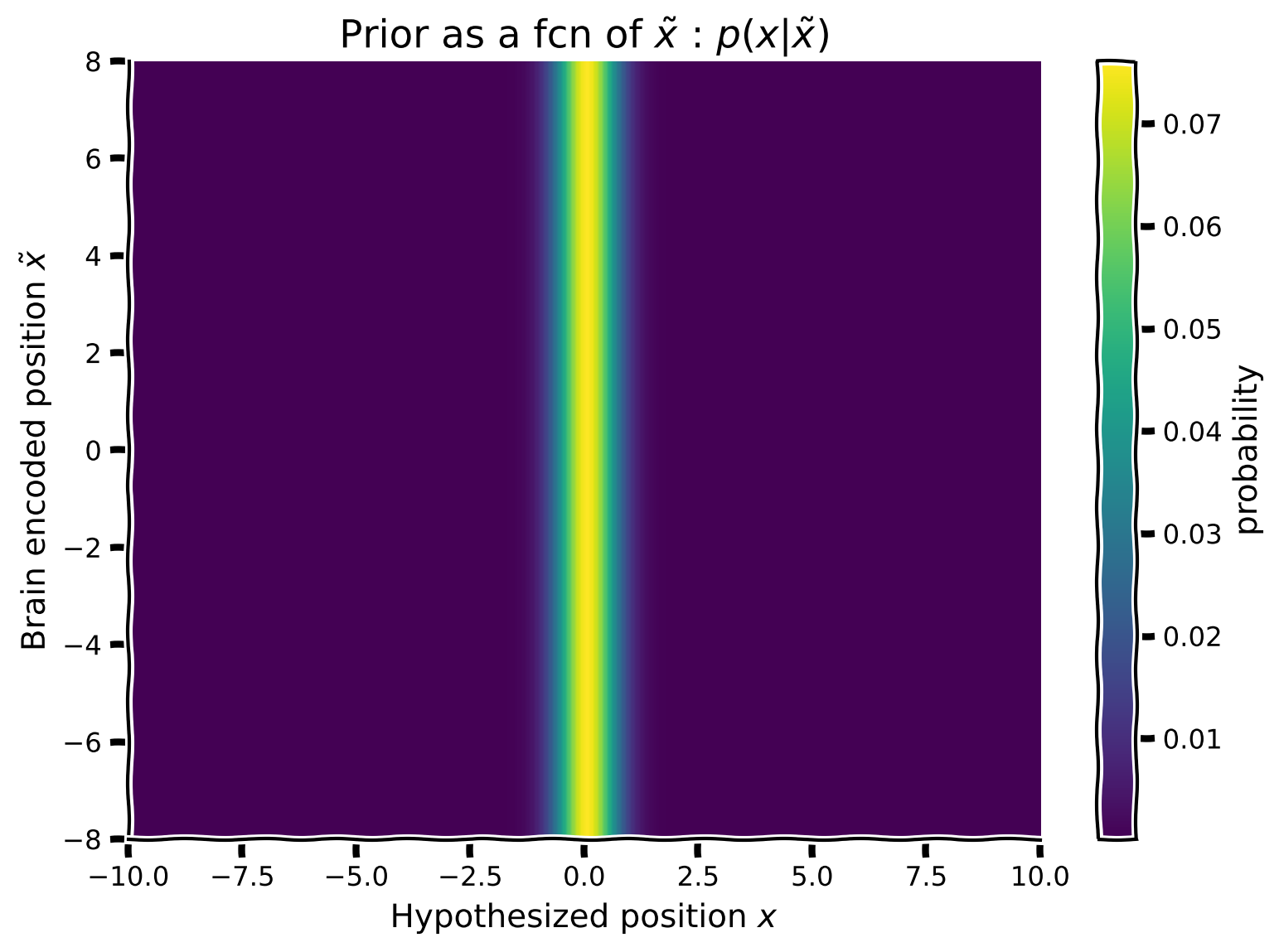
As in Tutorial 2, we want to create a prior that will describe the participants’ prior knowledge that, 95% of the time sounds come from a common position around the puppet, while during the remaining 5% of the time, they arise from another independent position. We will embody this information into a prior using a mixture of Gaussians. For visualization reasons, we will create a prior that has the same shape (form) as the likelihood array we created in the previous exercise. That is, we want to create a mixture of Gaussian prior as a function of the brain-encoded stimulus \(\tilde x\). Since the prior does not change as a function of \(\tilde x\) it will be identical for each row of the prior 2D array.

Using the equation for the Gaussian my_gaussian:

Generate a Gaussian \(Common\) with mean 0 and standard deviation 0.5
Generate another Gaussian \(Independent\) with mean 0 and standard deviation 10
Combine the two Gaussians (Common + Independent) to make a new prior by mixing the two Gaussians with mixing parameter \(p_{independent}\) = 0.05. Make it such that the peakier Gaussian has 95% of the weight (don’t forget to normalize afterwards)
This will be the first row of your prior 2D array
Now repeat this for varying brain encodings \(\tilde x\). Since the prior does not depend on \(\tilde x\), you can just repeat the prior for each \(\tilde x\) (hint: use np.tile) that row prior to making an array of 1,000 (i.e., hypothetical_stim.shape[0]) row-priors.
Plot the matrix using the function plot_myarray() already pre-written and commented-out in your script.

Coding Exercise 2: Implement the prior array#

def calculate_prior_array(x_points, stim_array, p_indep,
                          prior_mean_common=.0, prior_sigma_common=.5,
                          prior_mean_indep=.0, prior_sigma_indep=10):
  """
      'common' stands for common
      'indep' stands for independent
  """

  prior_common = my_gaussian(x_points, prior_mean_common, prior_sigma_common)
  prior_indep = my_gaussian(x_points, prior_mean_indep, prior_sigma_indep)
  ############################################################################
  ## Insert your code here to:
  ##      - Create a mixture of gaussian priors from 'prior_common'
  ##        and 'prior_indep' with mixing parameter 'p_indep'
  ##      - normalize
  ##      - repeat the prior array and reshape it to make a 2D array
  ##        of 1000 rows of priors (Hint: use np.tile() and np.reshape())
  ## remove the raise below to test your function
  raise NotImplementedError("You need to complete the function!")
  ############################################################################
  prior_mixed = ...
  prior_mixed /= ...  # normalize

  prior_array = np.tile(...).reshape(...)
  return prior_array


x = np.arange(-10, 10, 0.1)
p_independent = .05
prior_array = calculate_prior_array(x, hypothetical_stim, p_independent)
plot_myarray(prior_array,
             'Hypothesized position $x$', 'Brain encoded position $\~x$',
             'Prior as a fcn of $\~x$ : $p(x|\~x)$')

Click for solution

Example output:

Submit your feedback#

Section 3: Bayes rule and Posterior array#

Video 3: Posterior array#

Submit your feedback#

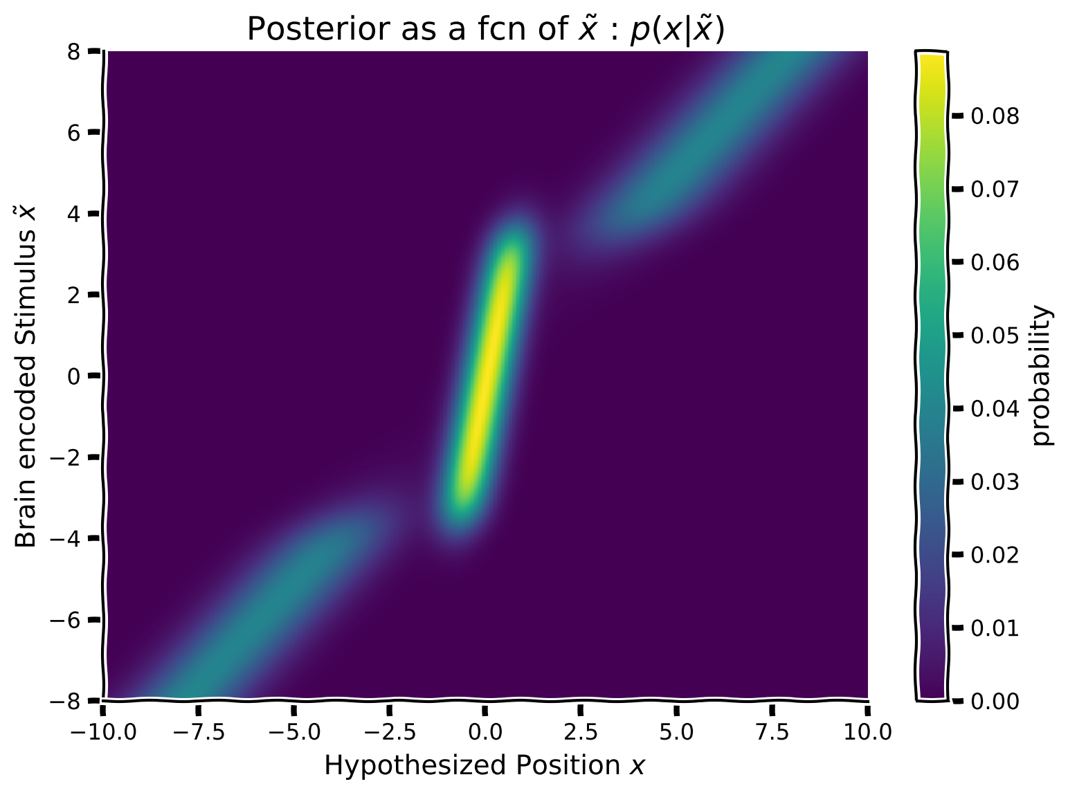
We now want to calculate the posterior using Bayes Rule. Since we have already created a likelihood and a prior for each brain encoded position \(\tilde x\), all we need to do is to multiply them row-wise. That is, each row of the posterior array will be the posterior resulting from the multiplication of the prior and likelihood of the same equivalent row.

Mathematically:

(366)#\[\begin{equation} Posterior\left[i, :\right] \propto Likelihood\left[i, :\right] \odot Prior\left[i, :\right] \end{equation}\]

where \(\odot\) represents the Hadamard Product (i.e., element-wise multiplication) of the corresponding prior and likelihood row vectors i from each matrix.

Follow these steps to build the posterior as a function of the brain encoded stimulus \(\tilde x\):

For each row of the prior and likelihood (i.e., each possible brain encoding \(\tilde x\)), fill in the posterior matrix so that every row of the posterior array represents the posterior density for a different brain encode \(\tilde x\).
Plot the array using the function plot_myarray() already pre-written and commented-out in your script

Optional:

Do you need to operate on one element–or even one row–at a time? NumPy operations can often process an entire matrix in a single “vectorized” operation. This approach is often much faster and much easier to read than an element-by-element calculation. Try to write a vectorized version that calculates the posterior without using any for-loops. Hint: look at np.sum and its keyword arguments.

Coding Exercise 3: Calculate the posterior as a function of the hypothetical stimulus \(x\)#

def calculate_posterior_array(prior_array, likelihood_array):
  ############################################################################
  ## Insert your code here to:
  ##      - calculate the 'posterior_array' from the given
  ##        'prior_array', 'likelihood_array'
  ##      - normalize
  ## remove the raise below to test your function
  raise NotImplementedError("You need to complete the function!")
  ############################################################################
  posterior_array = ...
  posterior_array /= ...  # normalize each row separately

  return posterior_array


posterior_array = calculate_posterior_array(prior_array, likelihood_array)
plot_myarray(posterior_array,
             'Hypothesized Position $x$',
             'Brain encoded Stimulus $\~x$',
             'Posterior as a fcn of $\~x$ : $p(x | \~x)$')

Click for solution

Example output:

Submit your feedback#

Section 4: Estimating the position \(\hat x\)#

Video 4: Binary decision matrix#

Submit your feedback#

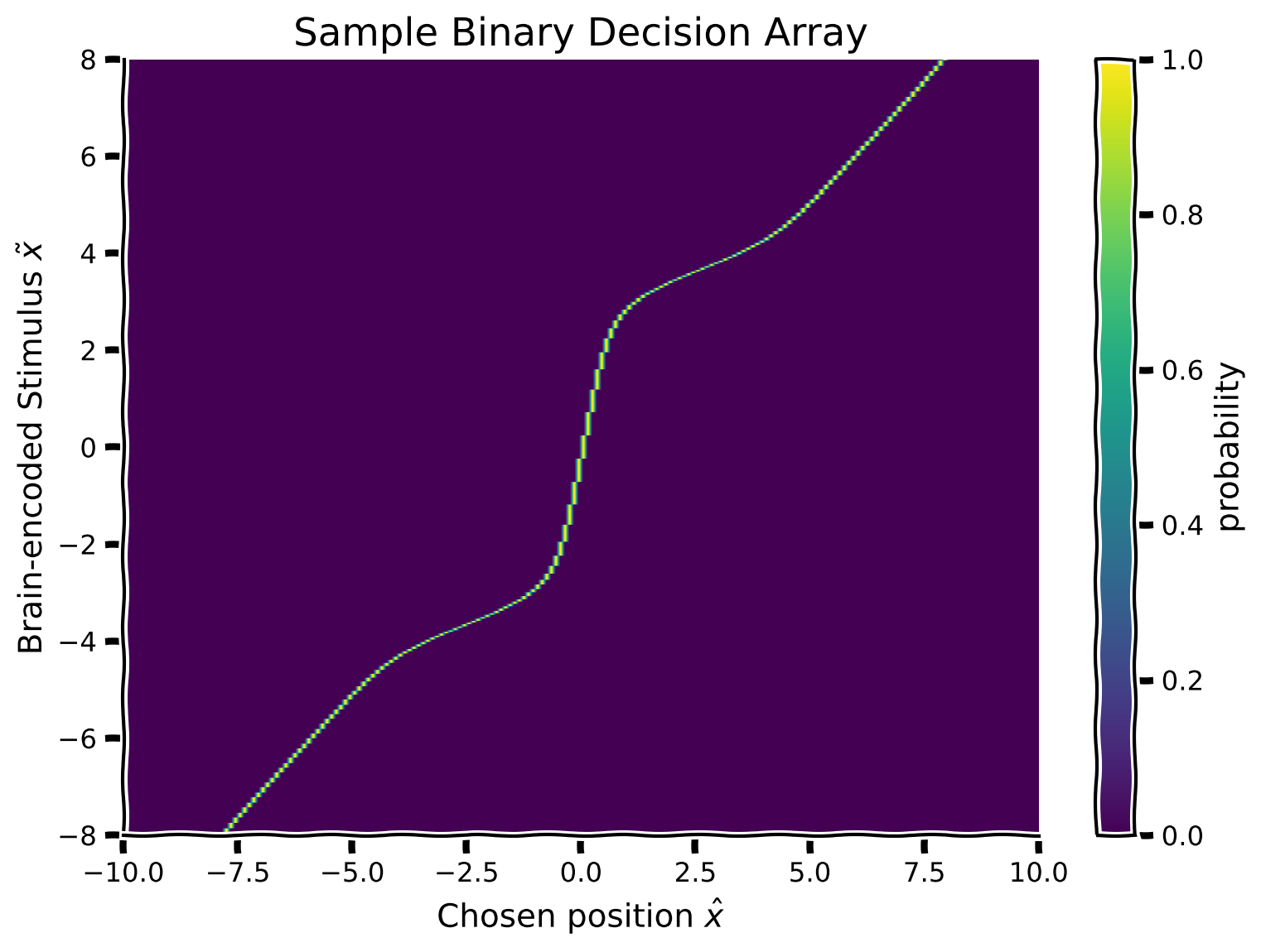
Now that we have a posterior distribution (for each possible brain encoding \(\tilde x\))that represents the brain’s estimated stimulus position: \(p(x|\tilde x)\), we want to make an estimate (response) of the sound location \(\hat x\) using the posterior distribution. This would represent the subject’s estimate if their (for us as experimentalists unobservable) brain encoding took on each possible value.

This effectively encodes the decision that a participant would make for a given brain encoding \(\tilde x\). In this exercise, we make the assumption that participants take the mean of the posterior (decision rule) as a response estimate for the sound location (use the function moments_myfunc() provided to calculate the mean of the posterior).

Using this knowledge, we will now represent \(\hat x\) as a function of the encoded stimulus \(\tilde x\). This will result in a 2D binary decision array. To do so, we will scan the posterior matrix (i.e. row-wise), and set the array cell value to 1 at the mean of the row-wise posterior.

Suggestions

For each brain encoding \(\tilde x\) (row of the posterior array), calculate the mean of the posterior, and set the corresponding cell of the binary decision array to 1. (e.g., if the mean of the posterior is at position 0, then set the cell with x_column == 0 to 1).
Plot the matrix using the function plot_myarray() already pre-written and commented-out in your script

Coding Exercise 4: Calculate the estimated response as a function of the hypothetical stimulus x#

def calculate_binary_decision_array(x_points, posterior_array):

  binary_decision_array = np.zeros_like(posterior_array)

  for i in range(len(posterior_array)):
    ########################################################################
    ## Insert your code here to:
    ##      - For each hypothetical stimulus x (row of posterior),
    ##        calculate the mean of the posterior using the provided function
    ##        `moments_myfunc()`, and set the corresponding cell of the
    ##        Binary Decision array to 1.
    ##        Hint: you can run 'help(moments_myfunc)' to see the docstring
    ## remove the raise below to test your function
    raise NotImplementedError("You need to complete the function!")
    ########################################################################
    # calculate mean of posterior using 'moments_myfunc'
    mean, _, _ = ...
    # find the position of mean in x_points (closest position)
    idx = ...
    binary_decision_array[i, idx] = 1

  return binary_decision_array


binary_decision_array = calculate_binary_decision_array(x, posterior_array)
plot_myarray(binary_decision_array,
             'Chosen position $\hat x$', 'Brain-encoded Stimulus $\~ x$',
             'Sample Binary Decision Array')

Click for solution

Example output:

Submit your feedback#

Section 5: Probabilities of encoded stimuli#

Video 5: Input array#

Submit your feedback#

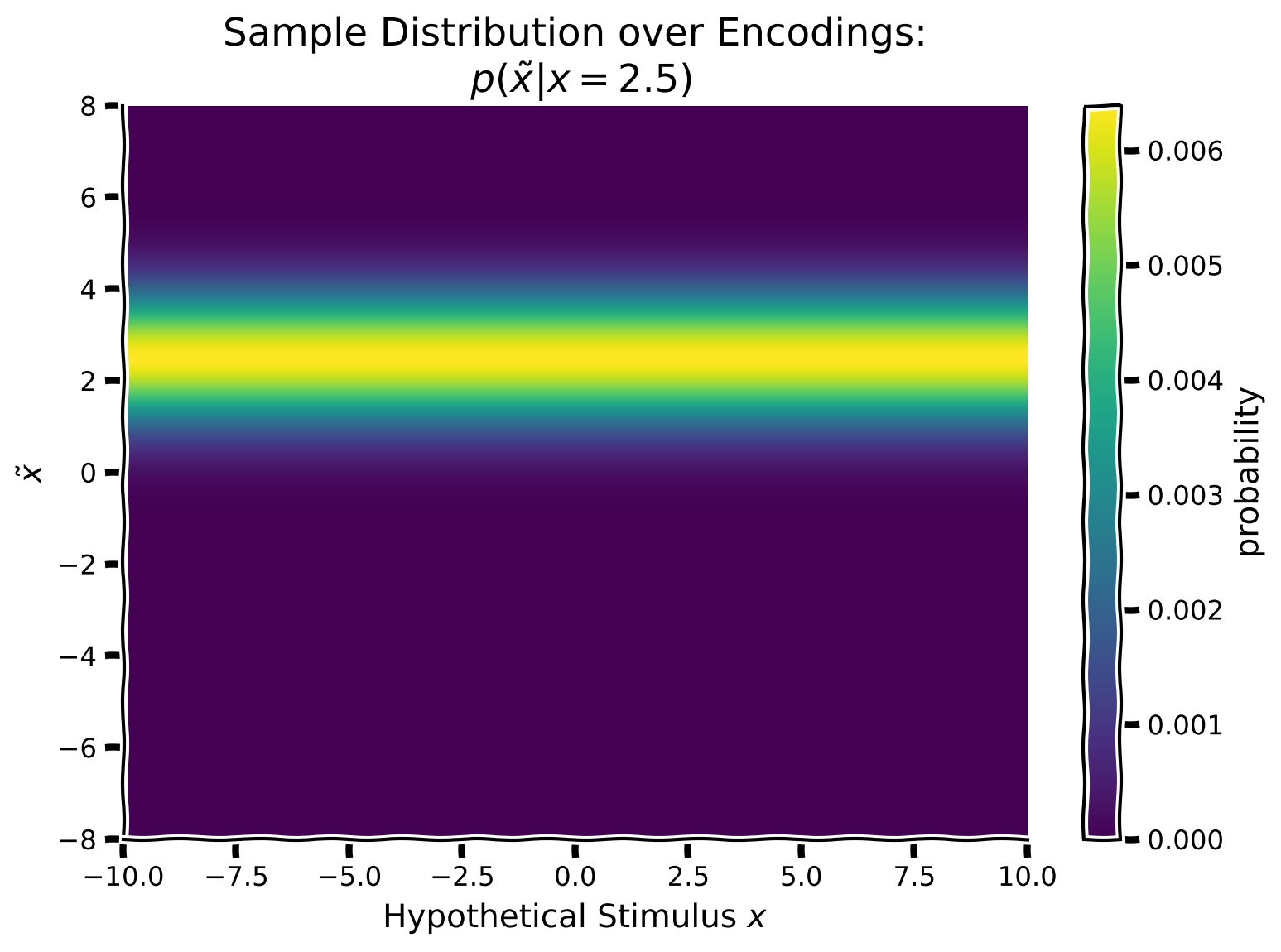
Because we as experimentalists can not know the encoding \(\tilde x\) of the stimulus \(x\) that we do know, we had to compute the binary decision array for each possible encoding.

First, however, we need to calculate how likely each possible encoding is given the true stimulus. That is, we will now create a Gaussian centered around the true presented stimulus, with \(\sigma = 1\), and repeat that Gaussian distribution across as a function of potentially encoded values \(\tilde x\). That is, we want to make a column gaussian centered around the true presented stimulus, and repeat this column Gaussian across all hypothetical stimulus values \(x\).

This effectively encodes the distribution of the brain-encoded stimulus (one single stimulus, which we as experimentalists know) and enables us to link the true stimulus \(x\), to potential encodings \(\tilde x\).

Suggestions

For this exercise, we will assume the true stimulus is presented at direction 2.5

Create a Gaussian likelihood with \(\mu = 2.5\) and \(\sigma = 1.0\)
Make this the first column of your array and repeat that column to fill in the true presented stimulus input as a function of hypothetical stimulus locations.
Plot the array using the function plot_myarray() already pre-written and commented-out in your script.

Coding Exercise 5: Generate an input as a function of hypothetical stimulus x#

def generate_input_array(x_points, stim_array, posterior_array,
                         mean=2.5, sigma=1.):

  input_array = np.zeros_like(posterior_array)
  ########################################################################
  ## Insert your code here to:
  ##      - Generate a gaussian centered on the true stimulus 2.5
  ##        and sigma = 1. for each column
  ## remove the raise below to test your function
  raise NotImplementedError("You need to complete the function!")
  ########################################################################
  for i in range(len(x_points)):
    input_array[:, i] = ...

  return input_array


input_array = generate_input_array(x, hypothetical_stim, posterior_array)
plot_myarray(input_array,
             'Hypothetical Stimulus $x$', '$\~x$',
             'Sample Distribution over Encodings:\n $p(\~x | x = 2.5)$')

Click for solution

Example output:

Submit your feedback#

Section 6: Normalization and expected estimate distribution#

Video 6: Marginalization#

Submit your feedback#

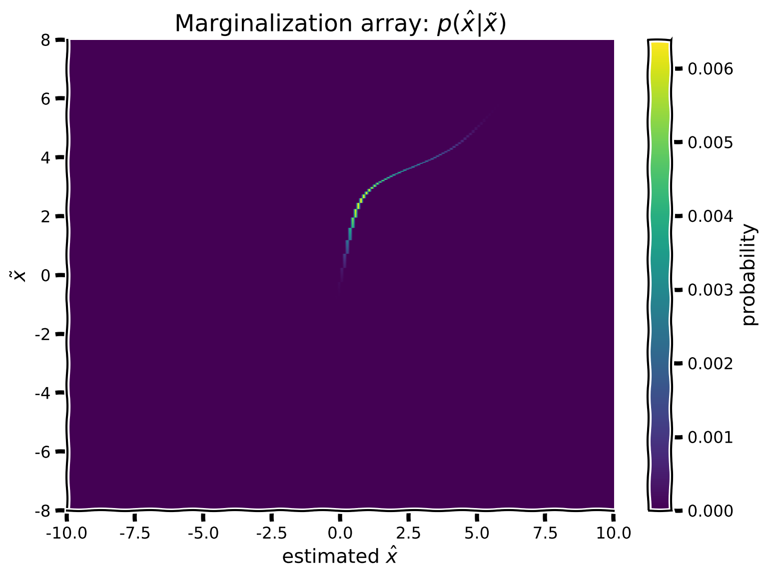
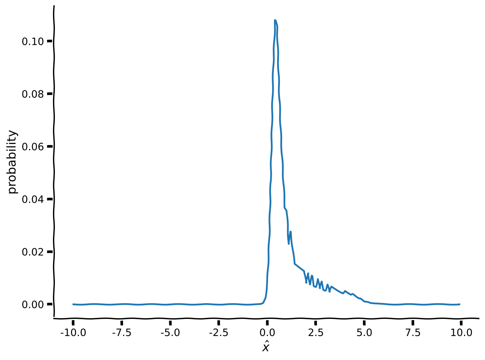
Now that we have a true stimulus \(x\) and a way to link it to potential encodings, we will be able to calculate the distribution of encodings and ultimately estimates. To integrate over all possible hypothetical values of \(\tilde x\) we marginalize, that is, we first compute the dot-product from the true presented stimulus and our binary decision array and then sum over \(x\).

Mathematically, this means that we want to compute:

(367)#\[\begin{eqnarray} \text{Marginalization Array} = \text{Input Array} \odot \text{Binary Decision Array} \end{eqnarray}\]

(368)#\[\begin{eqnarray} \text{Marginal} = \int_{\tilde x} \text{Marginalization Array} \end{eqnarray}\]

Since we are performing integration over discrete values using arrays for visualization purposes, the integration reduces to a simple sum over \(\tilde x\).

Suggestions

For each row of the input and binary arrays, calculate product of the two and fill in the 2D marginal array.
Plot the result using the function plot_myarray() already pre-written and commented-out in your script
Calculate and plot the marginal over x using the code snippet commented out in your script
- Note how the limitations of numerical integration create artifacts on your marginal

Coding Exercise 6: Implement the marginalization matrix#

def my_marginalization(input_array, binary_decision_array):

  ############################################################################
  ## Insert your code here to:
  ##  - Compute 'marginalization_array' by multiplying pointwise the Binary
  ##    decision array over hypothetical stimuli and the Input array
  ##  - Compute 'marginal' from the 'marginalization_array' by summing over x
  ##    (hint: use np.sum() and only marginalize along the columns)
  ## remove the raise below to test your function
  raise NotImplementedError("You need to complete the function!")
  ############################################################################

  marginalization_array = ...
  marginal = ... # note axis
  marginal /= ... # normalize

  return marginalization_array, marginal


marginalization_array, marginal = my_marginalization(input_array, binary_decision_array)

plot_myarray(marginalization_array,
             'estimated $\hat x$',
             '$\~x$',
             'Marginalization array: $p(\^x | \~x)$')
plt.figure()
plt.plot(x, marginal)
plt.xlabel('$\^x$')
plt.ylabel('probability')
plt.show()

Click for solution

Example output:

Submit your feedback#

Generate some data#

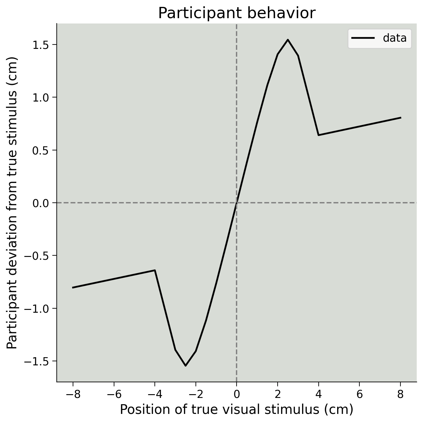
We have seen how to calculate the posterior and marginalize to remove \(\tilde x\) and get \(p(\hat{x} \mid x)\). Next, we will generate some artificial data for a single participant using the generate_data() function provided, and mixing parameter \(p_{independent} = 0.1\).

Our goal in the next exercise will be to recover that parameter. These parameter recovery experiments are a powerful method for planning and debugging Bayesian analyses–if you cannot recover the given parameters, something has gone wrong! Note that this value for \(p_{independent}\) is not quite the same as our prior, which used \(p_{independent} = 0.05.\) This lets us test out the complete model.

Please run the code below to generate some synthetic data. You do not need to edit anything, but check that the plot below matches what you would expect from the video.

#

Run the ‘generate_data’ function (this cell)#

../../../_images/8b9f7cc76421b33907a9804e4405fdb1bc2e9dcd8d0b8226c9021e62f5c6aa90.png

Section 7: Model fitting#

Video 7: Log likelihood#

Submit your feedback#

Now that we have generated some data, we will attempt to recover the parameter \(p_{independent}\) that was used to generate it.

We have provided you with an incomplete function called my_Bayes_model_mse() that needs to be completed to perform the same computations you have performed in the previous exercises but over all the participant’s trial, as opposed to a single trial.

The likelihood has already been constructed; since it depends only on the hypothetical stimuli, it will not change. However, we will have to implement the prior matrix, since it depends on \(p_{independent}\). We will therefore have to recompute the posterior, input and the marginal in order to get \(p(\hat{x} \mid x)\).

Using \(p(\hat{x} \mid x)\), we will then compute the negative log-likelihood for each trial and find the value of \(p_{independent}\) that minimizes the negative log-likelihood (i.e. maximizes the log-likelihood. See the model fitting tutorials for a refresher).

In this experiment, we assume that trials are independent from one another. This is a common assumption–and it’s often even true! It allows us to define negative log-likelihood as:

(369)#\[\begin{equation} -LL = - \sum_i \log p(\hat{x}_i \mid x_i) \end{equation}\]

where \(\hat{x}_i\) is the participant’s response for trial \(i\), with presented stimulus \(x_i\)

Complete the function my_Bayes_model_mse, we’ve already pre-completed the function to give you the prior, posterior, and input arrays on each trial
Compute the marginalization array as well as the marginal on each trial
Compute the negative log likelihood using the marginal and the participant’s response
Using the code snippet commented out in your script to loop over possible values of \(p_{independent}\)

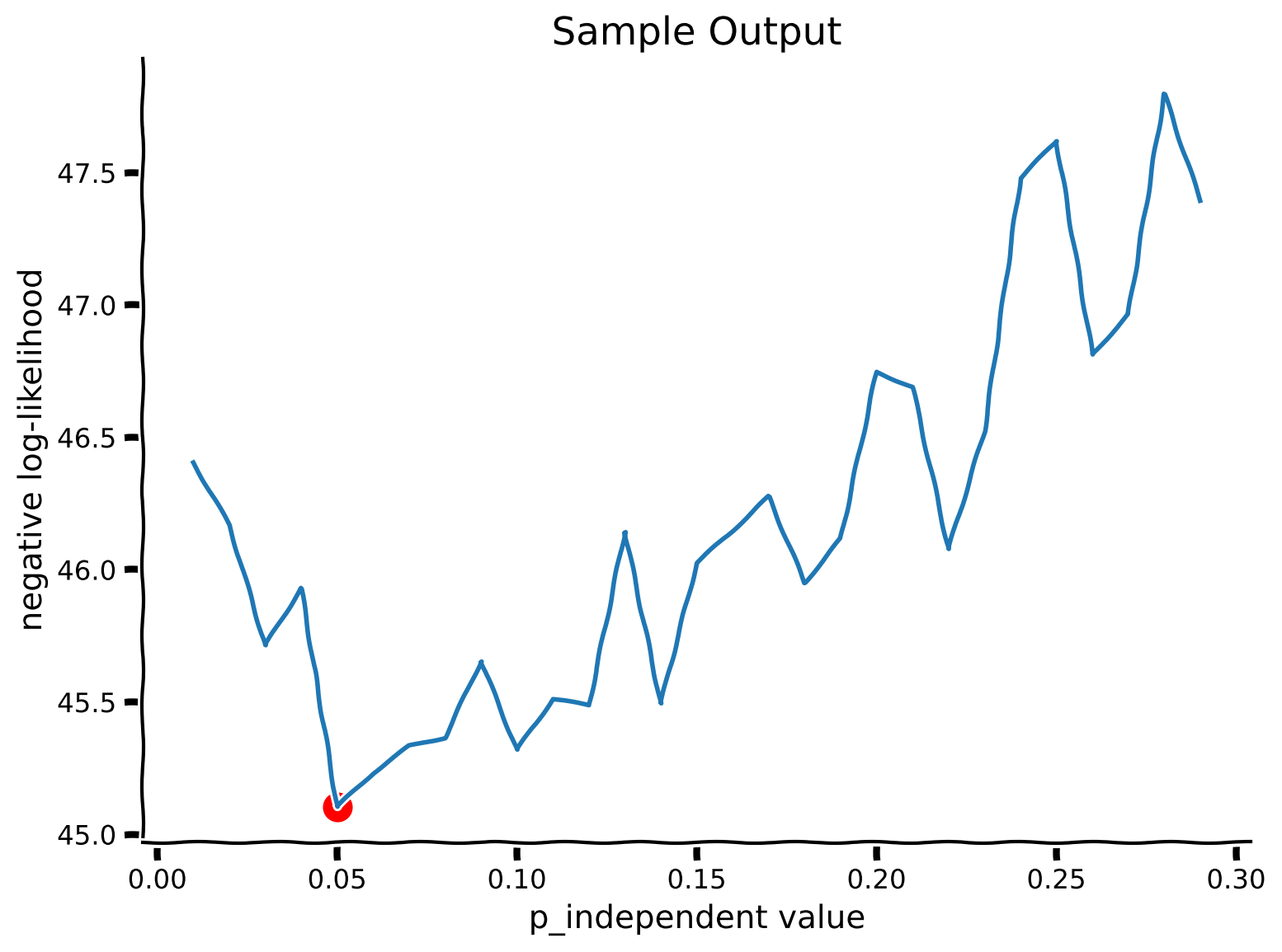
Coding Exercise 7: Fitting a model to generated data#

def my_Bayes_model_mse(params):
  """
  Function fits the Bayesian model from Tutorial 4

  Args :
      params (list of positive floats):  parameters used by the model
      (params[0]  = posterior scaling)

  Returns :
      (scalar) negative log-likelihood :sum of log probabilities
  """
  # Create the prior array
  p_independent=params[0]
  prior_array = calculate_prior_array(x,
                                      hypothetical_stim,
                                      p_independent,
                                      prior_sigma_indep= 3.)
  # Create posterior array
  posterior_array = calculate_posterior_array(prior_array, likelihood_array)
  # Create Binary decision array
  binary_decision_array = calculate_binary_decision_array(x, posterior_array)
  # we will use trial_ll (trial log likelihood) to register each trial
  trial_ll = np.zeros_like(true_stim)

  # Loop over stimuli
  for i_stim in range(len(true_stim)):
    # create the input array with true_stim as mean
    input_array = np.zeros_like(posterior_array)
    for i in range(len(x)):
      input_array[:, i] = my_gaussian(hypothetical_stim, true_stim[i_stim], 1)
      input_array[:, i] = input_array[:, i] / np.sum(input_array[:, i])

    # calculate the marginalizations
    marginalization_array, marginal = my_marginalization(input_array,
                                                         binary_decision_array)
    action = behaviour[i_stim]
    idx = np.argmin(np.abs(x - action))
    ########################################################################
    ## Insert your code here to:
    ##      - Compute the log likelihood of the participant
    ## remove the raise below to test your function
    raise NotImplementedError("You need to complete the function!")
    ########################################################################
    # Get the marginal likelihood corresponding to the action
    marginal_nonzero = ... + np.finfo(float).eps  # avoid log(0)
    trial_ll[i_stim] = np.log(marginal_nonzero)

  neg_ll = -trial_ll.sum()

  return neg_ll


plot_my_bayes_model(my_Bayes_model_mse)

Click for solution

Example output:

Submit your feedback#

Section 8: Summary#

Video 8: Outro#

Submit your feedback#

Congratulations! You found \(p_{independent}\), the parameter that describes how much weight subjects assign to the same-cause vs. independent-cause origins of a sound. In the preceding notebooks, we went through the entire Bayesian analysis pipeline:

developing a model
simulating data, and
using Bayes’ Rule and marginalization to recover a hidden parameter from the data

This example was simple, but the same principles can be used to analyze datasets with many hidden variables and complex priors and likelihoods.

Bonus Tutorial: Fitting to data

Contents

Bonus Tutorial: Fitting to data#

Tutorial objectives#

Setup#

Install and import feedback gadget#

Figure Settings#

Plotting functions#

Helper Functions#

Introduction#

Video 1: Intro#

Submit your feedback#

Section 1: Likelihood array#

Coding Exercise 1: Implement the auditory likelihood as a function of true stimulus position#

Submit your feedback#

Section 2: Causal mixture of Gaussian prior#

Video 2: Prior array#

Submit your feedback#

Coding Exercise 2: Implement the prior array#

Submit your feedback#

Section 3: Bayes rule and Posterior array#

Video 3: Posterior array#

Submit your feedback#

Coding Exercise 3: Calculate the posterior as a function of the hypothetical stimulus \(x\)#

Submit your feedback#

Section 4: Estimating the position \(\hat x\)#

Video 4: Binary decision matrix#

Submit your feedback#

Coding Exercise 4: Calculate the estimated response as a function of the hypothetical stimulus x#

Submit your feedback#

Section 5: Probabilities of encoded stimuli#

Video 5: Input array#

Submit your feedback#

Coding Exercise 5: Generate an input as a function of hypothetical stimulus x#

Submit your feedback#

Section 6: Normalization and expected estimate distribution#

Video 6: Marginalization#

Submit your feedback#

Coding Exercise 6: Implement the marginalization matrix#

Submit your feedback#

Generate some data#

#

Run the ‘generate_data’ function (this cell)#

Section 7: Model fitting#

Video 7: Log likelihood#

Submit your feedback#

Coding Exercise 7: Fitting a model to generated data#

Submit your feedback#

Section 8: Summary#

Video 8: Outro#

Submit your feedback#