Bonus Tutorial: Spike-timing dependent plasticity (STDP)

Bonus Tutorial: Spike-timing dependent plasticity (STDP)#

Week 2, Day 3: Biological Neuron Models

By Neuromatch Academy

Content creators: Qinglong Gu, Songtin Li, John Murray, Richard Naud, Arvind Kumar

Content reviewers: Spiros Chavlis, Lorenzo Fontolan, Richard Gao, Matthew Krause

Production editors: Gagana B, Spiros Chavlis

Tutorial Objectives#

In this tutorial, we will focus on building a model of a synapse in which its synaptic strength changes as a function of the relative timing (i.e., time difference) between the spikes of the presynaptic and postsynaptic neurons, respectively. This change in the synaptic weight is known as spike-timing dependent plasticity (STDP).

Our goals for this tutorial are to:

build a model of synapse that show STDP
study how correlations in input spike trains influence the distribution of synaptic weights

Towards these goals, we will model the presynaptic input as Poisson type spike trains. The postsynaptic neuron will be modeled as an LIF neuron (see Tutorial 1).

Throughout this tutorial, we assume that a single postsynaptic neuron is driven by \(N\) presynaptic neurons. That is, there are \(N\) synapses, and we will study how their weights depend on the statistics or the input spike trains and their timing with respect to the spikes of the postsynaptic neuron.

Setup#

Install and import feedback gadget#

# Import libraries
import matplotlib.pyplot as plt
import numpy as np
import time

Figure Settings#

Plotting functions#

Show code cell source Hide code cell source

# @title Plotting functions
def my_raster_plot(range_t, spike_train, n):
  """Generates poisson trains

  Args:
    range_t     : time sequence
    spike_train : binary spike trains, with shape (N, Lt)
    n           : number of Poisson trains plot

  Returns:
    Raster_plot of the spike train
  """

  # Find the number of all the spike trains
  N = spike_train.shape[0]

  # n should be smaller than N:
  if n > N:
    print('The number n exceeds the size of spike trains')
    print('The number n is set to be the size of spike trains')
    n = N

  # Raster plot
  i = 0
  while i <= n:
    if spike_train[i, :].sum() > 0.:
      t_sp = range_t[spike_train[i, :] > 0.5]  # spike times
      plt.plot(t_sp, i * np.ones(len(t_sp)), 'k|', ms=10, markeredgewidth=2)
    i += 1
  plt.xlim([range_t[0], range_t[-1]])
  plt.ylim([-0.5, n + 0.5])
  plt.xlabel('Time (ms)')
  plt.ylabel('Neuron ID')
  plt.show()


def my_example_P(pre_spike_train_ex, pars, P):
  """Generates two plots (raster plot and LTP vs time plot)

  Args:
    pre_spike_train_ex     : spike-train
    pars : dictionary with the parameters
    P : LTP ratio

  Returns:
    my_example_P returns a rastert plot (top),
    and a LTP ratio across time (bottom)
  """
  spT = pre_spike_train_ex
  plt.figure(figsize=(7, 6))
  plt.subplot(211)
  color_set = ['red', 'blue', 'black', 'orange', 'cyan']
  for i in range(spT.shape[0]):
    t_sp = pars['range_t'][spT[i, :] > 0.5]   # spike times
    plt.plot(t_sp, i*np.ones(len(t_sp)), '|',
             color=color_set[i],
             ms=10, markeredgewidth=2)
  plt.xlabel('Time (ms)')
  plt.ylabel('Neuron ID')
  plt.xlim(0, 200)

  plt.subplot(212)
  for k in range(5):
    plt.plot(pars['range_t'], P[k, :], color=color_set[k], lw=1.5)
  plt.xlabel('Time (ms)')
  plt.ylabel('P(t)')
  plt.xlim(0, 200)

  plt.tight_layout()
  plt.show()


def mySTDP_plot(A_plus, A_minus, tau_stdp, time_diff, dW):
  plt.figure()
  plt.plot([-5 * tau_stdp, 5 * tau_stdp], [0, 0], 'k', linestyle=':')
  plt.plot([0, 0], [-A_minus, A_plus], 'k', linestyle=':')

  plt.plot(time_diff[time_diff <= 0], dW[time_diff <= 0], 'ro')
  plt.plot(time_diff[time_diff > 0], dW[time_diff > 0], 'bo')

  plt.xlabel(r't$_{\mathrm{pre}}$ - t$_{\mathrm{post}}$ (ms)')
  plt.ylabel(r'$\Delta$W', fontsize=12)
  plt.title('Biphasic STDP', fontsize=12, fontweight='bold')
  plt.show()

Helper functions#

Section 1: Spike-timing dependent plasticity (STDP)#

Video 1: STDP#

Submit your feedback#

Model of STDP#

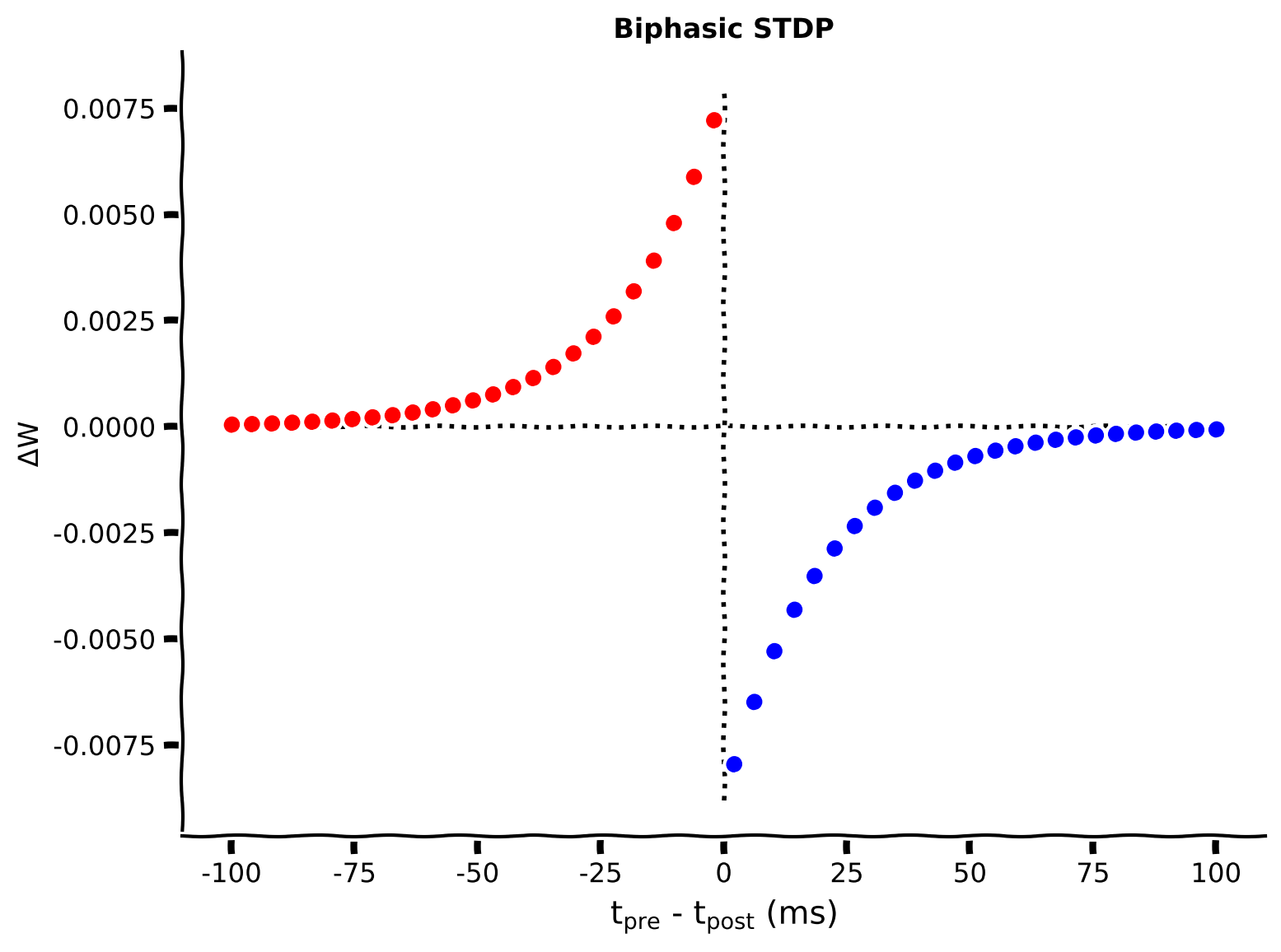
The phenomenology of STDP is generally described as a biphasic exponentially decaying function. That is, the instantaneous change in weights is given by:

(298)#\[\begin{eqnarray} & \Delta W &=& A_+ e^{ (t_{pre}-t_{post})/\tau_+} &\text{if} \hspace{5mm} t_{post} > t_{pre}& \\ & \Delta W &=& -A_- e^{- (t_{pre}-t_{post})/\tau_-} &\text{if} \hspace{5mm} t_{post} < t_{pre}& \end{eqnarray}\]

where \(\Delta W\) denotes the change in the synaptic weight, \(A_+\) and \(A_-\) determine the maximum amount of synaptic modification (which occurs when the timing difference between presynaptic and postsynaptic spikes is close to zero), \(\tau_+\) and \(\tau_-\) determine the ranges of pre-to-postsynaptic interspike intervals over which synaptic strengthening or weakening occurs. Thus, \(\Delta W > 0 \) means that postsynaptic neuron spikes after the presynaptic neuron.

This model captures the phenomena that repeated occurrences of presynaptic spikes within a few milliseconds before postsynaptic action potentials lead to long-term potentiation (LTP) of the synapse, whereas repeated occurrences of presynaptic spikes after the postsynaptic ones lead to long-term depression (LTD) of the same synapse.

The latency between presynaptic and postsynaptic spike (\(\Delta t\)) is defined as:

(299)#\[\begin{equation} \Delta t = t_{\rm pre} - t_{\rm post} \end{equation}\]

where \(t_{\rm pre}\) and \(t_{\rm post}\) are the timings of the presynaptic and postsynaptic spikes, respectively.

Complete the following code to set the STDP parameters and plot the STDP function. Note that for simplicity, we assume \(\tau_{+} = \tau_{-} = \tau_{\rm stdp}\).

Coding Exercise 1A: Compute the STDP changes \(\Delta W\)#

Note, as shown above, the expression of \(\Delta W\) is different for \(t_{post}>t_{pre}\) and \(t_{post}<t_{pre}\). In the code, we use the parameter time_diff that describes the \(t_{pre}-t_{post}\), as given above.

After implementing the code, you can visualize the STDP kernel, which describes how much the synaptic weight will change given a latency between the presynaptic and postsynaptic spikes.

def Delta_W(pars, A_plus, A_minus, tau_stdp):
  """
  Plot STDP biphasic exponential decaying function

  Args:
    pars       : parameter dictionary
    A_plus     : (float) maximum amount of synaptic modification
                 which occurs when the timing difference between pre- and
                 post-synaptic spikes is positive
    A_minus    : (float) maximum amount of synaptic modification
                 which occurs when the timing difference between pre- and
                 post-synaptic spikes is negative
    tau_stdp   : the ranges of pre-to-postsynaptic interspike intervals
                 over which synaptic strengthening or weakening occurs

  Returns:
    dW         : instantaneous change in weights
  """
  #######################################################################
  ## TODO for students: compute dP, then remove the NotImplementedError #
  # Fill out when you finish the function
  raise NotImplementedError("Student exercise: compute dW, the change in weights!")
  #######################################################################
  # STDP change
  dW = np.zeros(len(time_diff))
  # Calculate dW for LTP
  dW[time_diff <= 0] = ...
  # Calculate dW for LTD
  dW[time_diff > 0] = ...

  return dW


pars = default_pars_STDP()
# Get parameters
A_plus, A_minus, tau_stdp = pars['A_plus'], pars['A_minus'], pars['tau_stdp']
# pre_spike time - post_spike time
time_diff = np.linspace(-5 * tau_stdp, 5 * tau_stdp, 50)

dW = Delta_W(pars, A_plus, A_minus, tau_stdp)
mySTDP_plot(A_plus, A_minus, tau_stdp, time_diff, dW)

Click for solution

Example output:

Submit your feedback#

Keeping track of pre- and postsynaptic spikes#

Since a neuron will receive numerous presynaptic spike inputs, in order to implement STDP by taking into account different synapses, we first have to keep track of the pre- and postsynaptic spike times throughout the simulation.

A convenient way to do this is to define the following equation for each postsynaptic neuron:

(300)#\[\begin{equation} \tau_{-} \frac{dM}{dt} = -M \end{equation}\]

and whenever the postsynaptic neuron spikes,

(301)#\[\begin{equation} M(t) = M(t) - A_{-} \end{equation}\]

This way \(M(t)\) tracks the number of postsynaptic spikes over the timescale \(\tau_{-}\).

Similarly, for each presynaptic neuron, we define:

(302)#\[\begin{equation} \tau_{+} \frac{dP}{dt} = -P \end{equation}\]

and whenever there is spike on the presynaptic neuron,

(303)#\[\begin{equation} P(t) = P(t) + A_{+} \end{equation}\]

The variables \(M(t)\) and \(P(t)\) are very similar to the equations for the synaptic conductances, i.e., \(g_{i}(t)\), except that they are used to keep track of pre- and postsynaptic spike times on a much longer timescale. Note that, \(M(t)\) is always negative, and \(P(t)\) is always positive. You can probably already guess that \(M\) is used to induce LTD and \(P\) to induce LTP because they are updated by \(A_{-}\) and \(A_{+}\), respectively.

Important note: \(P(t)\) depends on the presynaptic spike times. If we know the presynaptic spike times, \(P\) can be generated before simulating the postsynaptic neuron and the corresponding STDP weights.

Visualization of \(P\)#

Here, we will consider a scenario in which there is a single postsynaptic neuron connected to \(N\) presynaptic neurons.

For instance, we have one postsynaptic neuron which receives Poisson type spiking inputs from five presynaptic neurons.

We can simulate \(P\) for each one of the presynaptic neurons.

Coding Exercise 1B: Compute \(dP\)#

Here, yet again, we use the Euler scheme, which has been introduced several times in the previous tutorials.

Similar to the dynamics of the membrane potential in the LIF model, in a time step \(dt\), \(P(t)\) will decrease by an amount of \(\displaystyle{\frac{dt}{\tau_+}P(t)}\). Whereas, if a presynaptic spike arrives, \(P(t)\) will instantaneously increase by an amount of \(A_+\). Therefore,

(304)#\[\begin{equation} dP = -\displaystyle{\frac{dt}{\tau_+}P[t]} + A_+\cdot \text{sp_or_not}[t+dt] \end{equation}\]

where the \(\text{sp_or_not}\) is a binary variable, i.e., \(\text{sp_or_not}=1\) if there is a spike within \(dt\), and \(\text{sp_or_not}=0\) otherwise.

def generate_P(pars, pre_spike_train_ex):
  """
  track of pre-synaptic spikes

  Args:
    pars               : parameter dictionary
    pre_spike_train_ex : binary spike train input from
                         presynaptic excitatory neuron

  Returns:
    P                  : LTP ratio
  """

  # Get parameters
  A_plus, tau_stdp = pars['A_plus'], pars['tau_stdp']
  dt, range_t = pars['dt'], pars['range_t']
  Lt = range_t.size

  # Initialize
  P = np.zeros(pre_spike_train_ex.shape)
  for it in range(Lt - 1):
    #######################################################################
    ## TODO for students: compute dP, then remove the NotImplementedError #
    # Fill out when you finish the function
    raise NotImplementedError("Student exercise: compute P, the change of presynaptic spike")
    #######################################################################
    # Calculate the delta increment dP
    dP = ...
    # Update P
    P[:, it + 1] = P[:, it] + dP

  return P


pars = default_pars_STDP(T=200., dt=1.)
pre_spike_train_ex = Poisson_generator(pars, rate=10, n=5, myseed=2020)
P = generate_P(pars, pre_spike_train_ex)
my_example_P(pre_spike_train_ex, pars, P)

Click for solution

Example output:

Submit your feedback#

Section 2: Implementation of STDP#

Finally, to implement STDP in spiking networks, we will change the value of the peak synaptic conductance based on the presynaptic and postsynaptic timing, thus using the variables \(P(t)\) and \(M(t)\).

Each synapse \(i\) has its own peak synaptic conductance (\(\bar g_i\)), which may vary between \([0, \bar g_{max}]\), and will be modified depending on the presynaptic and postsynaptic timing.

When the \(i_{th}\) presynaptic neuron elicits a spike, its corresponding peak conductance is updated according to the following equation:

(305)#\[\begin{equation} \bar g_i = \bar g_i + M(t)\bar g_{max} \end{equation}\]

Note that, \(M(t)\) tracks the time since the last postsynaptic potential and is always negative. Hence, if the postsynaptic neuron spikes shortly before the presynaptic neuron, the above equation shows that the peak conductance will decrease.
When the postsynaptic neuron spikes, the peak conductance of each synapse is updated according to:

(306)#\[\begin{equation} \bar g_i = \bar g_i + P_i(t)\bar g_{max}, \forall i \end{equation}\]

Note that, \(P_i(t)\) tracks the time since the last spike of \(i_{th}\) pre-synaptic neuron and is always positive.

Thus, the equation given above shows that if the presynaptic neuron spikes before the postsynaptic neuron, its peak conductance will increase.

LIF neuron connected with synapses that show STDP#

In the following exercise, we connect \(N\) presynaptic neurons to a single postsynaptic neuron. We do not need to simulate the dynamics of each presynaptic neuron as we are only concerned about their spike times. So, we will generate \(N\) Poisson type spikes. Here, we will assume that all these inputs are excitatory.

We need to simulate the dynamics of the postsynaptic neuron as we do not know its spike times. We model the postsynaptic neuron as an LIF neuron receiving only excitatory inputs.

(307)#\[\begin{equation} \tau_m\frac{dV}{dt} = -(V-E_L) - g_E(t) (V(t)-E_E)\, \end{equation}\]

where the total excitatory synaptic conductance \(g_{E}(t)\) is given by:

(308)#\[\begin{equation} g_E(t) = \sum_{i=1}^{N} g_i(t) \end{equation}\]

While simulating STDP, it is important to make sure that \(\bar g_i\) never goes outside of its bounds.

Function for LIF neuron with STDP synapses#

Show code cell source Hide code cell source

# @title Function for LIF neuron with STDP synapses

def run_LIF_cond_STDP(pars, pre_spike_train_ex):
  """
  conductance-based LIF dynamics

  Args:
    pars               : parameter dictionary
    pre_spike_train_ex : spike train input from presynaptic excitatory neuron

  Returns:
    rec_spikes         : spike times
    rec_v              : mebrane potential
    gE                 : postsynaptic excitatory conductance
  """

  # Retrieve parameters
  V_th, V_reset = pars['V_th'], pars['V_reset']
  tau_m = pars['tau_m']
  V_init, V_L = pars['V_init'], pars['V_L']
  gE_bar, VE, tau_syn_E = pars['gE_bar'], pars['VE'], pars['tau_syn_E']
  gE_init = pars['gE_init']
  tref = pars['tref']
  A_minus, tau_stdp = pars['A_minus'], pars['tau_stdp']
  dt, range_t = pars['dt'], pars['range_t']
  Lt = range_t.size

  P = generate_P(pars, pre_spike_train_ex)

  # Initialize
  tr = 0.
  v = np.zeros(Lt)
  v[0] = V_init
  M = np.zeros(Lt)
  gE = np.zeros(Lt)
  gE_bar_update = np.zeros(pre_spike_train_ex.shape)
  gE_bar_update[:, 0] = gE_init  # note: gE_bar is the maximum value

  # simulation
  rec_spikes = []  # recording spike times
  for it in range(Lt - 1):
      if tr > 0:
          v[it] = V_reset
          tr = tr - 1
      elif v[it] >= V_th:   # reset voltage and record spike event
          rec_spikes.append(it)
          v[it] = V_reset
          M[it] = M[it] - A_minus
          gE_bar_update[:, it] = gE_bar_update[:, it] + P[:, it] * gE_bar
          id_temp = gE_bar_update[:, it] > gE_bar
          gE_bar_update[id_temp, it] = gE_bar
          tr = tref / dt

      # update the synaptic conductance
      M[it + 1] = M[it] - dt / tau_stdp * M[it]
      gE[it + 1] = gE[it] - (dt / tau_syn_E) * gE[it] + (gE_bar_update[:, it] * pre_spike_train_ex[:, it]).sum()
      gE_bar_update[:, it + 1] = gE_bar_update[:, it] + M[it]*pre_spike_train_ex[:, it]*gE_bar
      id_temp = gE_bar_update[:, it + 1] < 0
      gE_bar_update[id_temp, it + 1] = 0.

      # calculate the increment of the membrane potential
      dv = (-(v[it] - V_L) - gE[it + 1] * (v[it] - VE)) * (dt / tau_m)

      # update membrane potential
      v[it + 1] = v[it] + dv

  rec_spikes = np.array(rec_spikes) * dt

  return v, rec_spikes, gE, P, M, gE_bar_update

print(help(run_LIF_cond_STDP))

Help on function run_LIF_cond_STDP in module __main__:

run_LIF_cond_STDP(pars, pre_spike_train_ex)
    conductance-based LIF dynamics
    
    Args:
      pars               : parameter dictionary
      pre_spike_train_ex : spike train input from presynaptic excitatory neuron
    
    Returns:
      rec_spikes         : spike times
      rec_v              : mebrane potential
      gE                 : postsynaptic excitatory conductance

None

Evolution of excitatory synaptic conductance#

In the following, we will simulate an LIF neuron receiving input from \(N=300\) presynaptic neurons.

pars = default_pars_STDP(T=200., dt=1.)  # Simulation duration 200 ms
pars['gE_bar'] = 0.024                   # max synaptic conductance
pars['gE_init'] = 0.024                  # initial synaptic conductance
pars['VE'] = 0.                          # [mV] Synapse reversal potential
pars['tau_syn_E'] = 5.                   # [ms] EPSP time constant

# generate Poisson type spike trains
pre_spike_train_ex = Poisson_generator(pars, rate=10, n=300, myseed=2020)
# simulate the LIF neuron and record the synaptic conductance
v, rec_spikes, gE, P, M, gE_bar_update = run_LIF_cond_STDP(pars,
                                                           pre_spike_train_ex)

Figures of the evolution of synaptic conductance#

Run this cell to see the figures!

Think! 2A: Analyzing Synaptic Strength and Conductance Transformations#

In the above, even though all the presynaptic neurons have the same average firing rate, many of the synapses seem to have been weakened? Did you expect that?
Total synaptic conductance is fluctuating over time. How do you expect \(g_E\) to fluctuate if synapses did not show any STDP like behavior?
Do synaptic weights ever reach a stationary state when synapses show STDP?

Click for solution

Submit your feedback#

Distribution of synaptic weight#

From the example given above, we get an idea that some synapses depotentiate, but what is the distribution of the synaptic weights when synapses show STDP?

In fact, it is possible that even the synaptic weight distribution itself is a time-varying quantity. So, we would like to know how the distribution of synaptic weights evolves as a function of time.

To get a better estimate of the weight distribution and its time evolution, we will increase the presynaptic firing rate to \(15\)Hz and simulate the postsynaptic neuron for \(120\)s.

Functions for simulating a LIF neuron with STDP synapses#

Show code cell source Hide code cell source

# @title Functions for simulating a LIF neuron with STDP synapses


def example_LIF_STDP(inputrate=15., Tsim=120000.):
  """
  Simulation of a LIF model with STDP synapses

  Args:
    intputrate  :  The rate used for generate presynaptic spike trains
    Tsim        :  Total simulation time

  output:
    Interactive demo, Visualization of synaptic weights
  """

  pars = default_pars_STDP(T=Tsim,  dt=1.)
  pars['gE_bar'] = 0.024
  pars['gE_init'] = 0.014  # initial synaptic conductance
  pars['VE'] = 0.          # [mV]
  pars['tau_syn_E'] = 5.   # [ms]

  starttime = time.perf_counter()
  pre_spike_train_ex = Poisson_generator(pars, rate=inputrate, n=300,
                                         myseed=2020)  # generate Poisson trains
  v, rec_spikes, gE, P, M, gE_bar_update = run_LIF_cond_STDP(pars,
                                                             pre_spike_train_ex)  # simulate LIF neuron with STDP
  gbar_norm = gE_bar_update/pars['gE_bar']  # calculate the ratio of the synaptic conductance
  endtime = time.perf_counter()
  timecost = (endtime - starttime) / 60.

  print('Total simulation time is %.3f min' % timecost)

  my_layout.width = '620px'

  @widgets.interact(
      sample_time=widgets.FloatSlider(0.5, min=0., max=1., step=0.1,
                                      layout=my_layout)
  )


  def my_visual_STDP_distribution(sample_time=0.0):
    sample_time = int(sample_time * pars['range_t'].size) - 1
    sample_time = sample_time * (sample_time > 0)

    plt.figure(figsize=(8, 8))
    ax1 = plt.subplot(211)
    for i in range(50):
      ax1.plot(pars['range_t'][::1000] / 1000., gE_bar_update[i, ::1000], lw=1., alpha=0.7)

    ax1.axvline(1e-3 * pars['range_t'][sample_time], 0., 1., color='k', ls='--')
    ax1.set_ylim(0, 0.025)
    ax1.set_xlim(-2, 122)
    ax1.set_xlabel('Time (s)')
    ax1.set_ylabel(r'$\bar{g}$')

    bins = np.arange(-.05, 1.05, .05)
    g_dis, _ = np.histogram(gbar_norm[:, sample_time], bins)
    ax2 = plt.subplot(212)
    ax2.bar(bins[1:], g_dis, color='b', alpha=0.5, width=0.05)
    ax2.set_xlim(-0.1, 1.1)
    ax2.set_xlabel(r'$\bar{g}/g_{\mathrm{max}}$')
    ax2.set_ylabel('Number')
    ax2.set_title(('Time = %.1f s' % (1e-3 * pars['range_t'][sample_time])),
                  fontweight='bold')
    plt.show()


print(help(example_LIF_STDP))

Help on function example_LIF_STDP in module __main__:

example_LIF_STDP(inputrate=15.0, Tsim=120000.0)
    Simulation of a LIF model with STDP synapses
    
    Args:
      intputrate  :  The rate used for generate presynaptic spike trains
      Tsim        :  Total simulation time
    
    output:
      Interactive demo, Visualization of synaptic weights

None

Interactive Demo 2: Example of an LIF model with STDP#

Make sure you execute this cell to enable the widget!

Think! 2B: Effects of Increased Presynaptic Firing Rate#

Increase the firing rate (i.e., 30 Hz) of presynaptic neurons, and investigate the effect on the dynamics of synaptic weight distribution.

Click for solution

Submit your feedback#

Section 3: Effect of input correlations#

Thus far, we assumed that the input population was uncorrelated. What do you think will happen if presynaptic neurons were correlated?

In the following, we will modify the input such that first \(L\) neurons have identical spike trains while the remaining inputs are uncorrelated. This is a highly simplified model of introducing correlations. You can try to code your own model of correlated spike trains.

Function for LIF neuron with STDP synapses receiving correlated inputs#

Show code cell source Hide code cell source

# @title Function for LIF neuron with STDP synapses receiving correlated inputs


def example_LIF_STDP_corrInput(inputrate=20., Tsim=120000.):
  """
  A LIF model equipped with STDP synapses, receiving correlated inputs

  Args:
    intputrate      :  The rate used for generate presynaptic spike trains
    Tsim            :  Total simulation time

  Returns:
    Interactive demo: Visualization of synaptic weights
  """

  np.random.seed(2020)
  pars = default_pars_STDP(T=Tsim, dt=1.)
  pars['gE_bar'] = 0.024
  pars['VE'] = 0.                                # [mV]
  pars['gE_init'] = 0.024 * np.random.rand(300)  # initial synaptic conductance
  pars['tau_syn_E'] = 5.                         # [ms]

  starttime = time.perf_counter()
  pre_spike_train_ex = Poisson_generator(pars, rate=inputrate, n=300, myseed=2020)
  for i_pre in range(50):
    pre_spike_train_ex[i_pre, :] = pre_spike_train_ex[0, :]  # simple way to set input correlated
  v, rec_spikes, gE, P, M, gE_bar_update = run_LIF_cond_STDP(pars, pre_spike_train_ex) # simulate LIF neuron with STDP
  gbar_norm = gE_bar_update / pars['gE_bar']  # calculate the ratio of the synaptic conductance
  endtime = time.perf_counter()
  timecost = (endtime - starttime) / 60.

  print(f'Total simulation time is {timecost:.3f} min')

  my_layout.width = '620px'

  @widgets.interact(
      sample_time=widgets.FloatSlider(0.5, min=0., max=1., step=0.05,
                                      layout=my_layout)
  )


  def my_visual_STDP_distribution(sample_time=0.0):

    sample_time = int(sample_time * pars['range_t'].size) - 1
    sample_time = sample_time*(sample_time > 0)
    figtemp = plt.figure(figsize=(8, 8))
    ax1 = plt.subplot(211)
    for i in range(50):
      ax1.plot(pars['range_t'][::1000] / 1000.,
               gE_bar_update[i, ::1000], lw=1., color='r', alpha=0.7, zorder=2)

    for i in range(50):
      ax1.plot(pars['range_t'][::1000] / 1000.,
               gE_bar_update[i + 50, ::1000], lw=1., color='b',
               alpha=0.5, zorder=1)

    ax1.axvline(1e-3 * pars['range_t'][sample_time], 0., 1.,
                color='k', ls='--', zorder=2)
    ax1.set_ylim(0, 0.025)
    ax1.set_xlim(-2, 122)
    ax1.set_xlabel('Time (s)')
    ax1.set_ylabel(r'$\bar{g}$')
    legend=ax1.legend(['Correlated input', 'Uncorrelated iput'], fontsize=18,
                      loc=[0.92, -0.6], frameon=False)
    for color, text, item in zip(['r', 'b'], legend.get_texts(), legend.legend_handles):
      text.set_color(color)
      item.set_visible(False)

    bins = np.arange(-.05, 1.05, .05)
    g_dis_cc, _ = np.histogram(gbar_norm[:50, sample_time], bins)
    g_dis_dp, _ = np.histogram(gbar_norm[50:, sample_time], bins)

    ax2 = plt.subplot(212)
    ax2.bar(bins[1:], g_dis_cc, color='r', alpha=0.5, width=0.05)
    ax2.bar(bins[1:], g_dis_dp, color='b', alpha=0.5, width=0.05)
    ax2.set_xlim(-0.1, 1.1)
    ax2.set_xlabel(r'$\bar{g}/g_{\mathrm{max}}$')
    ax2.set_ylabel('Number')
    ax2.set_title(('Time = %.1f s' % (1e-3 * pars['range_t'][sample_time])),
                  fontweight='bold')
    plt.show()


print(help(example_LIF_STDP_corrInput))

Help on function example_LIF_STDP_corrInput in module __main__:

example_LIF_STDP_corrInput(inputrate=20.0, Tsim=120000.0)
    A LIF model equipped with STDP synapses, receiving correlated inputs
    
    Args:
      intputrate      :  The rate used for generate presynaptic spike trains
      Tsim            :  Total simulation time
    
    Returns:
      Interactive demo: Visualization of synaptic weights

None

Interactive Demo 3: LIF model with plastic synapses receiving correlated inputs#

Make sure you execute this cell to enable the widget!

Why do weights of uncorrelated neurons decrease when synapses show STDP?

Above, we notice that the synapses of correlated neurons (which spike together) were almost unaffected, but the weights of other neurons diminished. Why does this happen?

The reason is that the correlated presynaptic neurons have a higher chance of eliciting a spike in the postsynaptic neurons and that create a \(pre \rightarrow post\) pairing of spikes.

Think! 3: Applications of STDP#

Modify the code above and create two groups of correlated presynaptic neurons and test what happens to the weight distribution.
How can the above observations be used to create unsupervised learning? Could you imagine how we have to train a neuronal model enabled with STDP rule to identify input patterns?
What else can be done with this type of plasticity?

Click for solution

Submit your feedback#

Summary#

Hooray! You have just finished this loooong day! In this tutorial, we covered the concept of spike-timing dependent plasticity (STDP).

We managed to:

build a model of synapse that shows STDP.
study how correlations in input spike trains influence the distribution of synaptic weights.

Using presynaptic inputs as Poisson type spike trains, we modeled an LIF model with synapses equipped with STDP. We also studied the effect of correlated inputs on the synaptic strength!

Bonus Tutorial: Spike-timing dependent plasticity (STDP)

Contents

Bonus Tutorial: Spike-timing dependent plasticity (STDP)#

Tutorial Objectives#

Setup#

Install and import feedback gadget#

Figure Settings#

Plotting functions#

Helper functions#

Section 1: Spike-timing dependent plasticity (STDP)#

Video 1: STDP#

Submit your feedback#

Model of STDP#

Coding Exercise 1A: Compute the STDP changes \(\Delta W\)#

Submit your feedback#

Keeping track of pre- and postsynaptic spikes#

Visualization of \(P\)#

Coding Exercise 1B: Compute \(dP\)#

Submit your feedback#

Section 2: Implementation of STDP#

LIF neuron connected with synapses that show STDP#

Function for LIF neuron with STDP synapses#

Evolution of excitatory synaptic conductance#

Figures of the evolution of synaptic conductance#

Think! 2A: Analyzing Synaptic Strength and Conductance Transformations#

Submit your feedback#

Distribution of synaptic weight#

Functions for simulating a LIF neuron with STDP synapses#

Interactive Demo 2: Example of an LIF model with STDP#

Think! 2B: Effects of Increased Presynaptic Firing Rate#

Submit your feedback#

Section 3: Effect of input correlations#

Function for LIF neuron with STDP synapses receiving correlated inputs#

Interactive Demo 3: LIF model with plastic synapses receiving correlated inputs#

Think! 3: Applications of STDP#

Submit your feedback#

Summary#