Tutorial 4: Time-Frequency Methods

Tutorial 4: Time-Frequency Methods#

Week 2, Day 2: Time series and signal processing

By Neuromatch Academy (community contribution)

Content Creators: Anindita Basu, Johana Dominguez, Isaac Kinley

Content Reviewers: Sricharan Sunder, Gal Vishne, Richard Gao

Production Editors: Konstantine Tsafatinos

Tutorial Objectives#

Estimated timing of tutorial: 45 minutes

By the end of this tutorial, you should be able to:

explain why the PSD can miss temporal structure in non-stationary signals,
describe how the STFT restores timing information using local windows,
explain how window length and window shape create time-frequency trade-offs,
explain how wavelets redistribute that trade-off across frequencies,
describe how filtering and Hilbert transforms estimate instantaneous amplitude and phase,
explain how time-frequency concepts appear in neuroscience examples such as bursts, evoked/induced responses, phase locking, and ITPC.

The main conceptual progression for this tutorial is:

global spectrum → local spectrum → windowing and trade-offs → wavelets → amplitude/phase analyses.

Setup#

Run the setup cells once. They collect imports, figure styling, and helper functions used repeatedly throughout the tutorial.

Install and import feedback gadget#

Imports#

Figure Settings#

Plotting constants and helper functions#

Show code cell source Hide code cell source

# @title Plotting constants and helper functions

# Use Neuromatch's matplotlib style for global figure defaults.
# The colors below are semantic colors used to label tutorial-specific signals.
SIGNAL_COLOR = "#3E4A42"
PURPLE = "#7B6FD6"
GREEN = "#6CA66A"
ORANGE = "#E69F00"
BLUE = "#4C72B0"
MAROON = "#8F3C61"
LIGHT_GREEN = "#DCEFD8"

# Semantic colors used consistently throughout the tutorial.
TEN_HZ_COLOR = "lightgreen"
TWENTY_HZ_COLOR = "orange"
RECTANGULAR_FILTER_COLOR = "blue"

# Shared STFT/spectrogram parameters.
# These are used for the two Section 1 spectrograms and again in the
# STFT-versus-wavelet comparison, so students compare like with like.
STFT_NPERSEG = 128
STFT_OVERLAP_FRACTION = 0.5
STFT_NOVERLAP = int(STFT_OVERLAP_FRACTION * STFT_NPERSEG)
STFT_WINDOW = "hann"

# Set this to False for a student-release version where TODO cells should
# raise an error until the student fills them in. Keep True when you want
# the notebook to run from top to bottom.
RUN_WITH_SOLUTIONS = True

FIGSIZE_WIDE = (10.5, 3)
FIGSIZE_WIDE2 = (10.5, 3.5)
FIGSIZE_SINGLE = (5.5, 3)
FIGSIZE_GRID = (10.5, 6)
FIG_DPI = 130

# Font sizes
plt.rcParams["figure.titlesize"] = 13
plt.rcParams["axes.titlepad"] = 6
plt.rcParams["axes.labelsize"] = 10      # x/y axis labels
plt.rcParams["xtick.labelsize"] = 9      # x tick numbers
plt.rcParams["ytick.labelsize"] = 9      # y tick numbers
plt.rcParams["axes.titlesize"] = 11      # subplot titles
plt.rcParams["legend.fontsize"] = 9


def style_axis(ax, grid=True):
    """Apply light axis cleanup while preserving the Neuromatch style."""
    if grid:
        ax.grid(True, alpha=0.25)
    else:
        ax.grid(False)
    ax.spines["top"].set_visible(False)
    ax.spines["right"].set_visible(False)


def style_legend(ax, loc="best", fontsize=None):
    """Apply shared legend styling."""
    legend = ax.legend(loc=loc, fontsize=fontsize, frameon=True)
    if legend is not None:
        legend.get_frame().set_alpha(0.85)
    return legend


def plot_signal(ax, t, x, title="", xlabel="Time (s)", ylabel="Amplitude",
                color=SIGNAL_COLOR, label=None, linewidth=1.4):
    """Plot a time-domain signal."""
    ax.plot(t, x, color=color, linewidth=linewidth, label=label)
    ax.set_title(title)
    ax.set_xlabel(xlabel)
    ax.set_ylabel(ylabel)
    style_axis(ax)
    if label is not None:
        style_legend(ax)
    return ax


def plot_psd(ax, freqs, power, title="", fmax=None, color=PURPLE, label=None):
    """Plot a one-sided PSD."""
    if fmax is not None:
        mask = freqs <= fmax
        freqs = freqs[mask]
        power = power[mask]

    ax.semilogy(freqs, power + 1e-20, color=color, linewidth=1.5, label=label)
    ax.set_title(title)
    ax.set_xlabel("Frequency (Hz)")
    ax.set_ylabel("Power")
    style_axis(ax)
    if label is not None:
        style_legend(ax)
    return ax


def plot_fft_magnitude(ax, x, fs, title="", nfft=None, fmax=50,
                       color=PURPLE, label=None):
    """Plot a one-sided FFT magnitude spectrum."""
    if nfft is None:
        nfft = len(x)

    X = fft(x, n=nfft)
    freqs = fftfreq(nfft, 1 / fs)
    pos = freqs >= 0
    mask = freqs[pos] <= fmax

    ax.semilogy(
        freqs[pos][mask],
        np.abs(X[pos][mask]) + 1e-15,
        color=color,
        linewidth=1.4,
        label=label,
    )
    ax.set_title(title)
    ax.set_xlabel("Frequency (Hz)")
    ax.set_ylabel(r"Magnitude $|X(f)|$")
    ax.set_xlim(0, fmax)
    style_axis(ax)
    if label is not None:
        style_legend(ax)
    return X, freqs

Helper functions for wavelet-shape demos#

Show code cell source Hide code cell source

# @title Helper functions for wavelet-shape demos

def normalize_wavelet(w):
    """Normalize a wavelet to unit energy."""
    energy = np.sqrt(np.sum(np.abs(w) ** 2))
    if energy == 0:
        return w
    return w / energy


def morlet_wavelet(t, f0, n_cycles):
    """Complex Morlet wavelet."""
    sigma_t = n_cycles / (2 * np.pi * f0)
    envelope = np.exp(-t**2 / (2 * sigma_t**2))
    carrier = np.exp(2j * np.pi * f0 * t)
    return normalize_wavelet(envelope * carrier)


def mexican_hat_wavelet(t, f0, n_cycles):
    """Real-valued Mexican hat / Ricker-like wavelet."""
    sigma_t = n_cycles / (2 * np.pi * f0)
    u = t / sigma_t
    w = (1 - u**2) * np.exp(-u**2 / 2)
    return normalize_wavelet(w)


def gaussian_derivative_wavelet(t, f0, n_cycles):
    """First derivative of a Gaussian."""
    sigma_t = n_cycles / (2 * np.pi * f0)
    w = -t * np.exp(-t**2 / (2 * sigma_t**2))
    return normalize_wavelet(w)


def make_wavelet(t, wavelet_type="Morlet", f0=10, n_cycles=6):
    """Construct one of the wavelets used in the tutorial."""
    if wavelet_type == "Morlet":
        return morlet_wavelet(t, f0, n_cycles)
    if wavelet_type == "Mexican hat":
        return mexican_hat_wavelet(t, f0, n_cycles)
    if wavelet_type == "Gaussian derivative":
        return gaussian_derivative_wavelet(t, f0, n_cycles)
    raise ValueError(f"Unknown wavelet type: {wavelet_type}")


def plot_wavelet_demo(
    wavelet_type="Morlet",
    f0=10,
    n_cycles=6,
    duration=1.0,
    fs=1000,
    show_envelope=True,
    show_frequency=True,
):
    """Plot a wavelet in time and frequency."""
    plt.close("all")

    t_w = np.arange(-duration / 2, duration / 2, 1 / fs)
    w = make_wavelet(t_w, wavelet_type, f0, n_cycles)

    sigma_t = n_cycles / (2 * np.pi * f0)
    envelope = np.exp(-t_w**2 / (2 * sigma_t**2))
    envelope = envelope / np.max(envelope) * np.max(np.abs(w))

    if show_frequency:
        fig, axes = plt.subplots(
            1,
            2,
            figsize=FIGSIZE_WIDE,
            dpi=FIG_DPI,
            gridspec_kw={"width_ratios": [1.25, 1]},
        )
    else:
        fig, ax = plt.subplots(figsize=FIGSIZE_SINGLE, dpi=FIG_DPI)
        axes = [ax]

    ax = axes[0]
    if show_envelope:
        ax.fill_between(
            t_w,
            envelope,
            -envelope,
            color=LIGHT_GREEN,
            alpha=0.38,
            label="amplitude envelope",
        )
        ax.plot(t_w, envelope, color=GREEN, linewidth=1.5, alpha=0.95)
        ax.plot(t_w, -envelope, color=GREEN, linewidth=1.5, alpha=0.7)

    ax.plot(t_w, np.real(w), color=PURPLE, linewidth=2.5, label="real part")

    if np.iscomplexobj(w):
        ax.plot(
            t_w,
            np.imag(w),
            linestyle="--",
            color=BLUE,
            linewidth=2.3,
            label="imaginary part",
        )

    ax.axhline(0, color="#7A857A", linewidth=1.0, alpha=0.8)
    ax.set_title(f"{wavelet_type} wavelet", pad=14)
    ax.set_xlabel("Time (s)")
    ax.set_ylabel("Amplitude")
    style_axis(ax)
    style_legend(ax, loc="upper left", fontsize=9)

    ax.text(
        0.98,
        0.93,
        f"$f_0$ = {f0:.1f} Hz\ncycles = {n_cycles:.1f}\n$\\sigma_t$ = {sigma_t:.3f} s",
        transform=ax.transAxes,
        ha="right",
        va="top",
        bbox=dict(boxstyle="round,pad=0.35", facecolor="#F7FAF5", edgecolor="#CDBEEB"),
    )

    if show_frequency:
        ax = axes[1]
        W = np.fft.fft(w, n=8192)
        freqs = np.fft.fftfreq(len(W), d=1 / fs)
        pos = freqs >= 0

        ax.plot(freqs[pos], np.abs(W[pos]), color=PURPLE, linewidth=2.3)
        ax.axvline(f0, color=GREEN, linestyle="--", linewidth=1.8, label="center frequency")
        ax.set_xlim(0, min(50, fs / 2))
        ax.set_title("Frequency response", pad=14)
        ax.set_xlabel("Frequency (Hz)")
        ax.set_ylabel("Magnitude")
        style_axis(ax)
        style_legend(ax, loc="upper right", fontsize=9)

    plt.tight_layout()
    plt.show()


def make_synthetic_burst_signal(
    fs=500,
    duration=4.0,
    theta_freq=6,
    burst_freq=12,
    slow_drift_freq=3,
    burst_center=2.0,
    burst_width=0.3,
    noise_level=0.7,
    seed=1,
):
    """Generate a mixed signal with a hidden localized alpha-like burst."""
    t = np.arange(0, duration, 1 / fs)
    rng = np.random.default_rng(seed)

    noise = noise_level * rng.standard_normal(len(t))
    theta = 0.7 * np.sin(2 * np.pi * theta_freq * t)
    slow_drift = 0.6 * np.sin(2 * np.pi * slow_drift_freq * t)

    envelope = np.exp(-(t - burst_center) ** 2 / (2 * burst_width**2))
    alpha_burst = 1.5 * envelope * np.sin(2 * np.pi * burst_freq * t)

    x = theta + slow_drift + alpha_burst + noise

    return t, x, alpha_burst, envelope


def plot_synthetic_burst(t, x, alpha_burst=None, show_alpha=False):
    """Plot the mixed signal, optionally revealing the hidden burst component."""
    plt.close("all")

    fig, ax = plt.subplots(figsize=FIGSIZE_SINGLE, dpi=FIG_DPI)
    ax.plot(
        t,
        x,
        label="Observed mixed signal",
        color=SIGNAL_COLOR,
        linewidth=1.6,
        alpha=0.95,
    )

    if show_alpha and alpha_burst is not None:
        ax.plot(
            t,
            alpha_burst,
            label="Hidden localized signal",
            color=ORANGE,
            linewidth=2.8,
            alpha=0.98,
        )

    ax.axhline(0, color="#7A857A", linewidth=1.0, alpha=0.8)
    ax.set_xlabel("Time (s)")
    ax.set_ylabel("Amplitude")
    ax.set_title("Mixed signal with a hidden local component", pad=14)
    ax.set_xlim(t[0], t[-1])
    style_axis(ax)
    style_legend(ax, loc="upper left", fontsize=9)
    plt.tight_layout()
    plt.show()

Helper functions for Hilbert examples#

Show code cell source Hide code cell source

# @title Helper functions for Hilbert examples

def bandpass_filter(x, fs, low, high, order=4):
    """Band-pass filter using zero-phase Butterworth filtering."""
    sos = butter(order, [low, high], btype="bandpass", fs=fs, output="sos")
    return sosfiltfilt(sos, x)


def get_amp_phase(x):
    """Return instantaneous amplitude, phase, and analytic signal."""
    analytic = hilbert(x)
    amplitude = np.abs(analytic)
    phase = np.angle(analytic)
    return amplitude, phase, analytic


def plot_hilbert_snapshot(t, x, fs, time_point=1.25):
    """Interactive-friendly visualization of Hilbert amplitude and phase."""

    alpha_band = (8, 12)    # captures the 10 Hz burst
    beta_band = (18, 22)    # captures the 20 Hz burst

    alpha_filtered = bandpass_filter(x, fs, alpha_band[0], alpha_band[1])
    beta_filtered = bandpass_filter(x, fs, beta_band[0], beta_band[1])

    alpha_amp, alpha_phase, alpha_analytic = get_amp_phase(alpha_filtered)
    beta_amp, beta_phase, beta_analytic = get_amp_phase(beta_filtered)

    edge_crop = 0.5
    valid_mask = (t >= t[0] + edge_crop) & (t <= t[-1] - edge_crop)

    t_plot = t[valid_mask]
    x_plot = x[valid_mask]

    alpha_filtered_plot = alpha_filtered[valid_mask]
    alpha_amp_plot = alpha_amp[valid_mask]
    alpha_analytic_plot = alpha_analytic[valid_mask]

    beta_filtered_plot = beta_filtered[valid_mask]
    beta_amp_plot = beta_amp[valid_mask]
    beta_analytic_plot = beta_analytic[valid_mask]

    idx = np.argmin(np.abs(t_plot - time_point))

    raw_color = "#6E6E6E"
    alpha_color = GREEN      # 10 Hz burst: lightgreen
    beta_color = ORANGE      # 20 Hz burst: orange
    cycle_color = BLUE
    axis_color = "#7A857A"

    plt.close("all")
    fig, axes = plt.subplots(2, 2, figsize=FIGSIZE_GRID, dpi=FIG_DPI)
    # Alpha time series
    ax = axes[0, 0]
    ax.plot(t_plot, x_plot, color=raw_color, alpha=0.35, linewidth=1.3, label="raw")
    ax.plot(t_plot, alpha_filtered_plot, color=alpha_color, linewidth=1.9, label="alpha filtered")
    ax.plot(t_plot, alpha_amp_plot, color=alpha_color, linewidth=1.5, alpha=0.95, label="alpha amplitude")
    ax.plot(t_plot, -alpha_amp_plot, color=alpha_color, linewidth=1.5, alpha=0.55)
    ax.axvline(t_plot[idx], color=alpha_color, linestyle="--", linewidth=1.6)
    ax.axhline(0, color=axis_color, linewidth=0.9, alpha=0.75)
    ax.set_title("Alpha band: 8–12 Hz", pad=10)
    ax.set_xlabel("Time (s)")
    ax.set_ylabel("Amplitude")
    ax.set_xlim(t_plot[0], t_plot[-1])
    style_axis(ax)
    style_legend(ax, loc="upper right", fontsize=8)

    # Alpha analytic plane
    ax = axes[1, 0]
    ax.plot(
        np.real(alpha_analytic_plot),
        np.imag(alpha_analytic_plot),
        color=cycle_color,
        alpha=0.55,
        linewidth=1.7,
    )
    ax.scatter(
        np.real(alpha_analytic_plot[idx]),
        np.imag(alpha_analytic_plot[idx]),
        s=90,
        color=alpha_color,
        edgecolor="#2F3A32",
        linewidth=0.8,
        zorder=3,
    )
    ax.plot(
        [0, np.real(alpha_analytic_plot[idx])],
        [0, np.imag(alpha_analytic_plot[idx])],
        color=alpha_color,
        linewidth=2.0,
    )
    ax.axhline(0, color=axis_color, linewidth=0.9, alpha=0.75)
    ax.axvline(0, color=axis_color, linewidth=0.9, alpha=0.75)
    ax.set_title("Alpha analytic signal", pad=10)
    ax.set_xlabel("Real part")
    ax.set_ylabel("Imaginary part")
    ax.set_aspect("equal", adjustable="box")
    style_axis(ax)

    # Beta time series
    ax = axes[0, 1]
    ax.plot(t_plot, x_plot, color=raw_color, alpha=0.35, linewidth=1.3, label="raw")
    ax.plot(t_plot, beta_filtered_plot, color=beta_color, linewidth=1.9, label="beta filtered")
    ax.plot(t_plot, beta_amp_plot, color=beta_color, linewidth=1.5, alpha=0.95, label="beta amplitude")
    ax.plot(t_plot, -beta_amp_plot, color=beta_color, linewidth=1.5, alpha=0.55)
    ax.axvline(t_plot[idx], color=beta_color, linestyle="--", linewidth=1.6)
    ax.axhline(0, color=axis_color, linewidth=0.9, alpha=0.75)
    ax.set_title("Beta band: 18–22 Hz", pad=10)
    ax.set_xlabel("Time (s)")
    ax.set_ylabel("Amplitude")
    ax.set_xlim(t_plot[0], t_plot[-1])
    style_axis(ax)
    style_legend(ax, loc="upper right", fontsize=8)

    # Beta analytic plane
    ax = axes[1, 1]
    ax.plot(
        np.real(beta_analytic_plot),
        np.imag(beta_analytic_plot),
        color=cycle_color,
        alpha=0.55,
        linewidth=1.7,
    )
    ax.scatter(
        np.real(beta_analytic_plot[idx]),
        np.imag(beta_analytic_plot[idx]),
        s=90,
        color=beta_color,
        edgecolor="#2F3A32",
        linewidth=0.8,
        zorder=3,
    )
    ax.plot(
        [0, np.real(beta_analytic_plot[idx])],
        [0, np.imag(beta_analytic_plot[idx])],
        color=beta_color,
        linewidth=2.0,
    )
    ax.axhline(0, color=axis_color, linewidth=0.9, alpha=0.75)
    ax.axvline(0, color=axis_color, linewidth=0.9, alpha=0.75)
    ax.set_title("Beta analytic signal", pad=10)
    ax.set_xlabel("Real part")
    ax.set_ylabel("Imaginary part")
    ax.set_aspect("equal", adjustable="box")
    style_axis(ax)

    fig.suptitle(
        f"Instantaneous amplitude and phase at t = {t_plot[idx]:.2f} s",
        fontsize=16,
        y=1.02,
    )
    plt.tight_layout()
    plt.show()

Video 1: Time-frequency introduction#

Section 1: From frequency to time-frequency analysis#

Why is the Power Spectral Density unreliable for non-stationary signals?#

In Tutorial 2, we learned that the magnitude / power spectrum and Power Spectral Density (PSD) describes how the power in a signal is distributed across frequencies.

The power spectrum is the square of the magnitude spectrum, which is equivalent to computing a Fourier transform of the autocorrelation function of the global signal:

\[ S_X(f) = \int_{-\infty}^{\infty} R_X(\tau)\,e^{-i2\pi f\tau}\,d\tau. \]

where \(R_X(\tau)\) is the autocorrelation function of the signal \(X(t)\), and \(S_X(f)\) is the power spectral density at frequency \(f\).

For a stationary signal, power remains stable over time, making the PSD a useful summary.

But neural signals are often non-stationary: oscillations can appear and disappear as short transients, or change after a stimulus or an internal state transition.

The limitation of a global method like the PSD is that it averages power over the whole signal and cannot tell us when time-specific events occurred in non-stationary signals.

The Short-Time Fourier Transform (STFT) and the spectrogram#

Instead of computing the (discrete) Fourier transform of the entire signal, we can first segment the signal into short sliding windows (optionally with overlap), and compute the Fourier transform of each window.

This is called the Short-Time Fourier Transform (STFT). The STFT is a local Fourier transform that preserves the time information of the signal. Expressed in mathematical terms, the STFT of a signal \(x(t)\) is defined as:

\[ X(\tau, f) = \int_{-\infty}^{\infty} x(t)\,w(t-\tau)\,e^{-i2\pi ft}\,dt. \]

Here, \(w(t-\tau)\) is a window function that selects the part of the signal near time point \(\tau\).

The pipeline looks like the following:

Taking the squared magnitude \(|X(\tau,f)|^2\) at all frequencies and time points gives a map called a spectrogram, which shows how power at each frequency changes over time.

Video 2: From frequency to time-frequency analysis#

Submit your feedback#

Warm-up: When global power spectrum fails, we need time-frequency analysis#

Here we investigate why relying only on a power spectrum (PSD) can be misleading for non-stationary signals.

We will simulate two signals and compare what the PSD and STFT/spectrogram reveal about them.

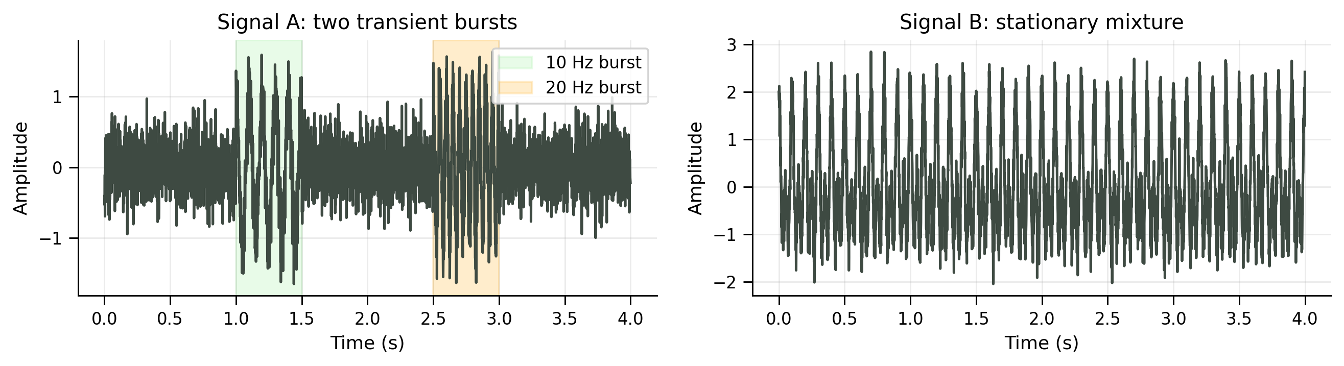
Generate two signals with the same frequencies but different temporal structure#

Signal A
  Burst 1: 1.0–1.5 s at 10 Hz
  Burst 2: 2.5–3.0 s at 20 Hz

Signal B
  10 Hz and 20 Hz are present simultaneously throughout the recording

Signal length: 4.0 s | sampling rate: 1000 Hz

Plot the simulated signals#

../../../_images/d567fd8c5722f172d4da37caddd76d6e3250e313bace610a422105349ae7084c.png

Compute and plot global PSDs#

../../../_images/030cad1ab2904ba3ebb93e6789bd42f967f046c340148c50db203c37f2daae49.png

Think!#

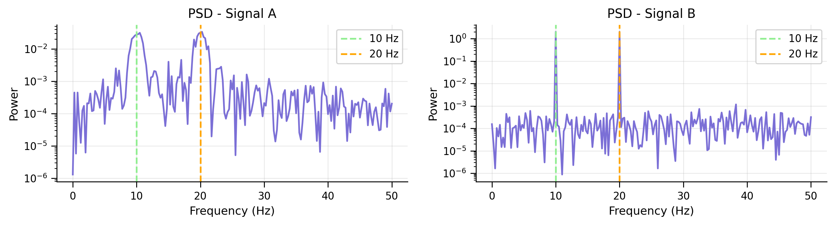
The peaks in both PSDs reveal that 10 Hz and 20 Hz are present. But the global PSD cannot answer:

whether the oscillations occurred continuously or as bursts,
when the bursts started and ended,
whether the 10 Hz and 20 Hz components overlapped in time.

To recover timing, we need a local spectral estimate. This motivates the STFT/spectrogram.

Submit your feedback#

Coding Exercise 1: Compute STFT with `scipy.signal.stft`#

In this exercise, you will complete one reusable function, compute_stft_spectrogram(). The only missing line is the SciPy call to signal.stft(), which takes care of the windowing and local Fourier transforms under the hood.

We will use the same STFT parameters throughout the tutorial (set in the CONSTANTS section at the top):

nperseg = 128
noverlap = int(0.5 * 128) = 64
window = "hann"

nperseg is the length of each segment (in samples), noverlap is the number of samples that overlap between sliding windows, and window is the type of window function applied to each segment.

After this function is complete, we will apply the STFT function to Signal A and Signal B and see whether it can recover time-specific information.

def compute_stft_spectrogram(
    x,
    fs,
    nperseg=STFT_NPERSEG,
    noverlap=STFT_NOVERLAP,
    window=STFT_WINDOW,
):
    """
    Compute a short-time Fourier transform spectrogram using scipy.signal.stft.

    Args:
      x (numpy array of floats): time-domain signal
      fs (float): sampling frequency in Hz
      nperseg (int): number of samples in each STFT window
      noverlap (int): number of samples shared by neighboring windows
      window (str): window type passed to scipy.signal.stft

    Returns:
      freqs (numpy array of floats): STFT frequency bins in Hz
      times (numpy array of floats): STFT time bins in seconds
      power_db (numpy array of floats): STFT power in dB, with shape
                                       (n_frequencies, n_times)
    """
    #################################################
    ## TODO for students: call scipy.signal.stft
    # Fill out function and remove
    raise NotImplementedError("Student exercise: call scipy.signal.stft!")
    #################################################

    # Compute the complex STFT coefficients
    freqs, times, Z = ...

    # Convert complex coefficients to power in dB.
    power = np.abs(Z) ** 2
    power_db = 10 * np.log10(power + 1e-12)

    return freqs, times, power_db

Click for solution

Use the completed STFT function: compare PSD and spectrograms#

Think!#

The spectrogram preserves information that the global power spectrum discards:

For Signal A, the spectrogram shows that the 10 Hz and 20 Hz components occur in different temporal windows.
For Signal B, the spectrogram shows continuous power at both frequencies.

This is the first lesson of the tutorial:

A time-frequency representation asks not only which frequencies are present, but also when they are present.

Submit your feedback#

Section 2: Window shape and spectral leakage#

Estimated timing to here from start of tutorial: 10 min

The STFT depends on windowing. A “window” not only selects a local segment of the signal, but multiplies the segment by a window shape. A naive window is a rectangular (or boxcar) window, which is the equivalent of simply grabbing a segment.

But as we will see, the choice of window shape in the time domain is important, as it determines the trade-offs in the frequency domain.

Video 3: Spectral leakage and windowing#

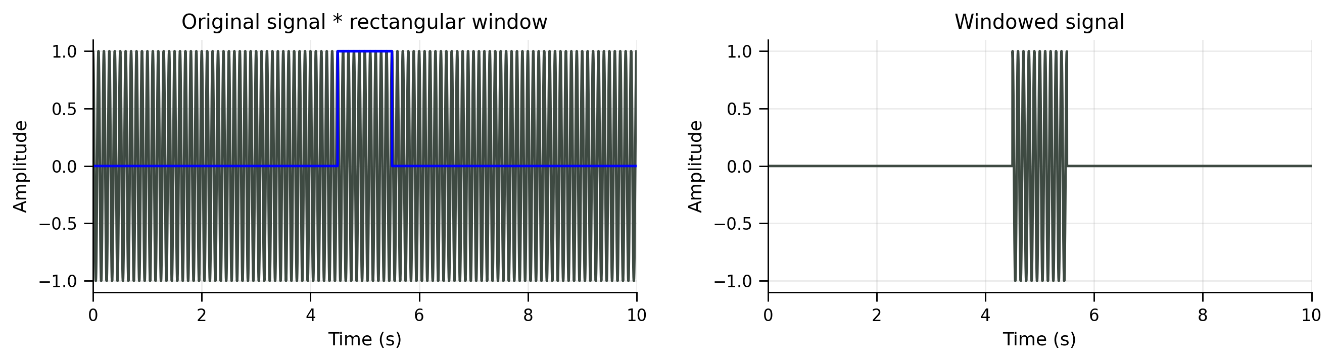
What is spectral leakage?#

Spectral leakage occurs when power from one frequency spreads into nearby frequencies in the estimated spectrum. This happens especially when the window boundaries introduce sharp discontinuities in the time domain.

Apply a rectangular window on a regular global signal#

../../../_images/41d9378213f88251c075fe313da47c21762f195b860e630eb4fac6f3c6bd2c2b.png

Compare FFT of the full signal and the windowed short segment#

../../../_images/0427d0ba790a333c6c5197960159af7e6204ba55970361d8aa455b830b6c9e6a.png

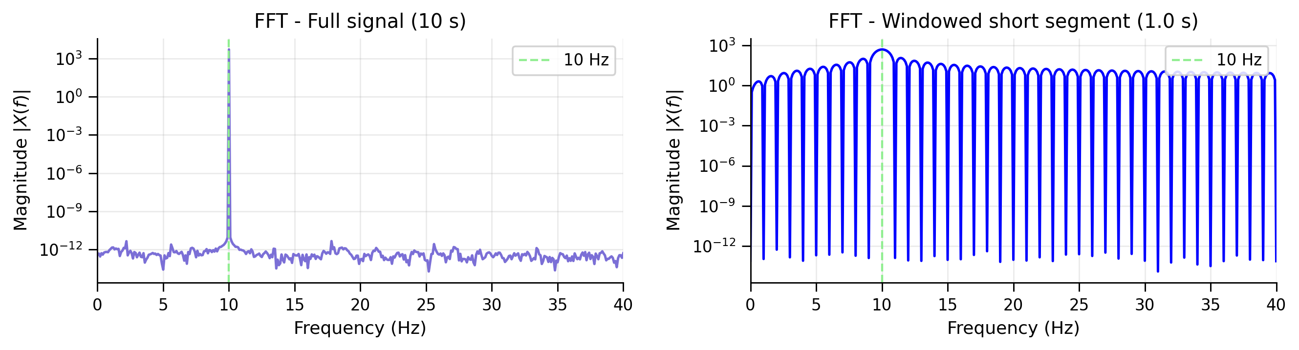
The “main lobe” in the center still detects the true frequency. But the “side lobes” reveal how much spectral leakage has occurred, i.e., phantom frequencies that are not actually present in the signal.

How can we reduce spectral leakage?#

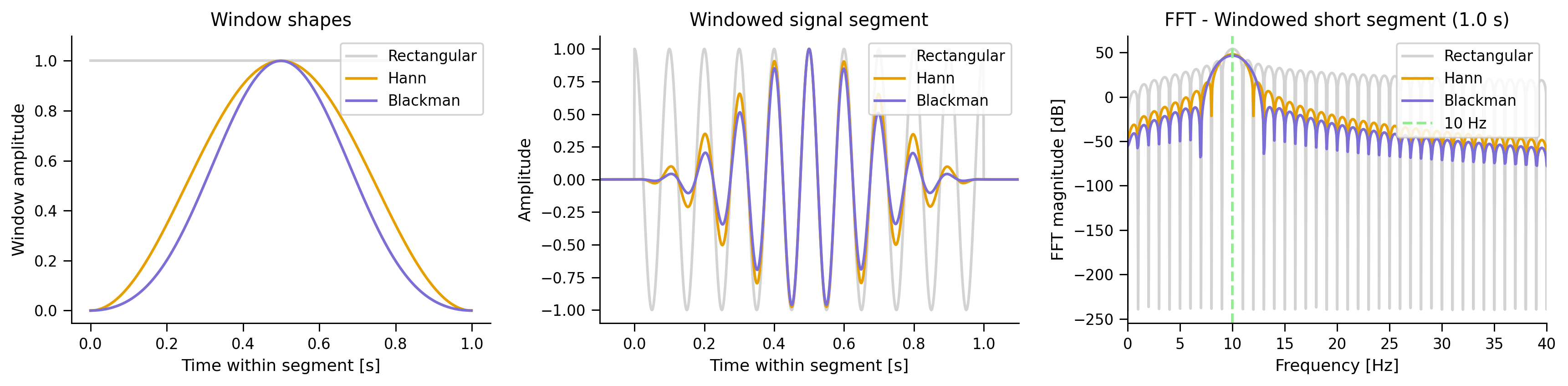
One common strategy is to taper the segment smoothly using a window such as a Hann or Blackman window. This reduces leakage in side lobes, but it also widens the main lobe.

We compare three windows:

Rectangular: narrowest main lobe, largest side lobes.
Hann: moderate main lobe, lower sidelobes.
Blackman: wider main lobe, strongest sidelobe suppression.

Compare leakage for common windows#

Show code cell source Hide code cell source

# @title Compare leakage for common windows
window_start = 4.5
window_duration = 1.0
window_end = window_start + window_duration

segment_mask = (t_leak >= window_start) & (t_leak < window_end)

t_segment = t_leak[segment_mask]
x_segment = x_leak[segment_mask]

n_window = len(x_segment)

rectangular = np.ones(n_window)
hann = np.hanning(n_window)
blackman = np.blackman(n_window)

windows = {
    "Rectangular": rectangular,
    "Hann": hann,
    "Blackman": blackman,
}

window_colors = {
    "Rectangular": "lightgrey",
    "Hann": ORANGE,
    "Blackman": PURPLE,
}

fig, axes = plt.subplots(1, 2, figsize=FIGSIZE_WIDE, dpi=FIG_DPI)

# Left: window shapes
for name, win in windows.items():
    axes[0].plot(
        t_segment - t_segment[0],
        win,
        color=window_colors[name],
        linewidth=1.6,
        label=name,
    )

axes[0].set_xlabel("Time within segment [s]")
axes[0].set_ylabel("Window amplitude")
axes[0].set_title("Window shapes")
axes[0].set_ylim(-0.05, 1.1)
style_legend(axes[0], loc="upper right", fontsize=9)

# Right: FFT of short windowed segment only
# Zero-padding: still using the short segment, but samples the frequency axis more finely
nfft = 16 * n_window

for name, win in windows.items():
    x_windowed_segment = x_segment * win

    freqs = np.fft.rfftfreq(nfft, d=1 / fs_leak)
    fft_vals = np.fft.rfft(x_windowed_segment, n=nfft)
    mag = np.abs(fft_vals)

    # dB scale without peak-normalizing
    mag_db = 20 * np.log10(mag + 1e-12)

    axes[1].plot(
        freqs,
        mag_db,
        color=window_colors[name],
        linewidth=1.6,
        label=name,
    )

axes[1].axvline(
    freq_leak,
    linestyle="--",
    color=TEN_HZ_COLOR,
    linewidth=1.6,
    label=f"{freq_leak} Hz",
)

axes[1].set_xlim(0, 40)
axes[1].set_xlabel("Frequency [Hz]")
axes[1].set_ylabel("FFT magnitude [dB]")
axes[1].set_title(f"FFT - Windowed short segment ({window_duration:.1f} s)")
style_legend(axes[1], loc="upper right", fontsize=9)

plt.tight_layout()
plt.show()

../../../_images/a96c73dc8061a8487ba5740bcc1ed357c97865c4724836860c347a3dd621e515.png

Think!#

Why does the rectangular window have sharp frequency resolution but large sidelobes?
If there is a second peak very close to the first peak, can it get hidden by the sidelobes of the window?

We see that there is a trade-off. If we use smoother windows to reduce spectral leakage in the STFT, we may fail to separate peaks at nearby frequencies.

The second message of this tutorial is that the choice of window shape introduces a trade-off between spectral leakage and frequency detection.

Submit your feedback#

Section 3: Window length and the time-frequency trade-off#

Estimated timing to here from start of tutorial: 18 min

Video 4: TF trade off#

Submit your feedback#

Recall from Tutorial 1 and 2 that the sampling rate and the number of samples determine the frequency resolution via the Nyquist theorem and the Discrete Fourier Transform: the longer the signal, the more fine-grained the frequency resolution.

The same principle holds for the STFT, where the length of the local window matters as well.

Window length determines an inherent trade-off between time resolution and frequency resolution:

A short window preserves precise timing, but it contains fewer cycles of the oscillation. This makes frequencies harder to detect.
A long window contains more cycles, so frequencies can be estimated more precisely. However, because the window spans a longer time interval, time precision is reduced.

This trade-off obeys the following uncertainty relationship inherent to Fourier transformation:

\[ \Delta t \, \Delta f \geq \frac{1}{4\pi} \]

A useful intuition is to imagine that you are listening to a piece of music and setting a metronome:

It is hard to tell whether the metronome is truly synchronized after listening to only a few seconds of beats. When you listen to the music and the metronome for a longer period, small differences accumulate and it becomes easier to detect a mismatch.

Short vs. long windows: how much evidence do we need?#

../../../_images/14b6942c9169ad8037a7028dd2f3a7a5770ab7e01e464928c8a77adc3c82f7ad.png

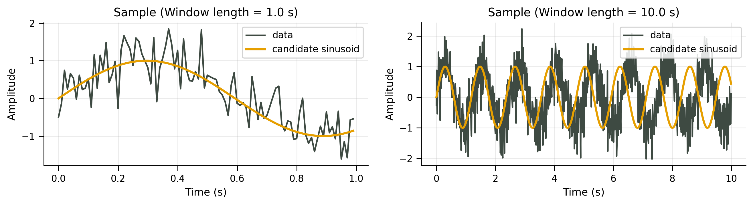
In the short window, the two rhythms look almost synchronized. There is not enough time for their small frequency difference to become obvious.

In the long window, the faster rhythm gradually drifts ahead. The same frequency difference becomes easier to detect because the evidence accumulates over more cycles.

Interactive Demo 1: Change the STFT window length#

Move the slider to change the STFT window length. Short windows localize the burst more sharply in time; long windows estimate frequency more cleanly but smear the burst across time.

Can you tell how many oscillatory bursts there are and when they occur, and at what frequency?

Demo#

Submit your feedback#

Section 4: Wavelets and frequency-dependent window lengths#

Estimated timing to here from start of tutorial: 25 min

The STFT uses the same window length for all frequencies, which means that we see more cycles of faster oscillations than slower oscillations. In other words, a fixed window length will collect different amounts of evidence for different frequencies and lead to an uneven time-frequency trade-off.

Wavelets use frequency-dependent window lengths and solve this issue.

What is a wavelet?#

A wavelet is a short-lived, wave-shaped function with positive and negative parts that cancel on average, but with nonzero energy. It is localized in both time and frequency.

Fourier analysis decomposes signals into infinitely extended sinusoids. Wavelet analysis decomposes signals into localized oscillatory “atoms”.

Video 5: Wavelets#

Submit your feedback#

Interactive Demo 2: Wavelet shapes and parameters#

Use the controls to see how wavelet type, center frequency, and number of cycles affect localization in time and frequency.

Demo 2#

The number of cycles controls how much evidence the wavelet gathers to estimate power at a frequency:

low cycles: precise timing, blurry frequency,
high cycles: precise frequency, blurry timing.

Wavelets do not eliminate the time-frequency trade-off. They redistribute it across frequencies.

Submit your feedback#

Coding Exercise 2: Apply Morlet wavelets with MNE-Python#

In this exercise, you will complete one reusable function, compute_morlet_power(). The only missing line is the call to the MNE-Python function tfr_array_morlet().

MNE-Python expects data with shape:

(n_epochs, n_channels, n_times)

Our signal is one epoch and one channel, so the function reshapes it with:

x[np.newaxis, np.newaxis, :]

After this function is complete, the next cell will call both compute_stft_spectrogram() and compute_morlet_power() to compare the STFT and wavelets on the same signal.

def compute_morlet_power(x, fs, freqs, n_cycles=12):
    """
    Compute Morlet wavelet power using mne.time_frequency.tfr_array_morlet.

    Args:
      x (numpy array of floats): time-domain signal
      fs (float): sampling frequency in Hz
      freqs (numpy array of floats): frequencies of interest in Hz
      n_cycles (float or array): number of cycles in the Morlet wavelet

    Returns:
      power_db (numpy array of floats): Morlet power in dB, with shape
                                       (n_frequencies, n_times)
    """

    # MNE expects shape: (n_epochs, n_channels, n_times)
    data_mne = x[np.newaxis, np.newaxis, :]

    #################################################
    ## TODO for students: call mne.time_frequency.tfr_array_morlet
    # Fill out function and remove
    raise NotImplementedError("Student exercise: call tfr_array_morlet!")
    #################################################

    # Compute power using MNE-Python
    power = ...


    # Remove the artificial epoch and channel dimensions.
    power = power[0, 0, :, :]

    # Convert power to dB.
    power_db = 10 * np.log10(power + 1e-12)

    return power_db

Click for solution

Compare STFT and Morlet wavelets for Signal A#

Think!#

For the low-frequency burst (10Hz), how does the time and frequency resolution compare between the STFT and wavelet spectrograms?
How precisely can the STFT localize the bursts in time and frequency?
What changes if you make the STFT window longer or shorter?
When would you use the STFT, and when would you consider using wavelets?

Submit your feedback#

What do neuroscientists actually do with STFT and wavelets?#

In real neural signals, power is often dynamic and transient.

Bursts#

A burst is a brief packet of oscillatory activity in a specific frequency band.

Examples:

Alpha burst (~8–12 Hz): often seen over visual areas; linked to attention, sensory gating, and eyes-closed/resting EEG or MEG.
Beta burst (~13–30 Hz): often studied in motor and cognitive control contexts.
Sleep spindle (~10–15 Hz): a classic burst-like oscillation during NREM sleep, linked to thalamocortical dynamics and memory consolidation.

Section 5: Hilbert transform#

Estimated timing to here from start of tutorial: 35 min

Sometimes we do not need a full time-frequency map. Instead, we may want to track moment-to-moment changes in the amplitude and phase of one rhythm, such as alpha.

What is the Hilbert transform?#

The Hilbert transform takes a real-valued oscillatory signal \(x(t)\) and creates a second copy of that signal in the imaginary plane that is phase-shifted by 90 degrees. Together, the original signal and the phase-shifted signal form a complex-valued signal \(z(t)\) known as the analytic signal:

\[z(t) = x(t) + i\,\mathcal{H}\{x(t)\}\]

We can visualize the analytic signal as a moving arrow in the complex plane:

\[z(t) = A(t)e^{i\phi(t)}\]

the angle \(\phi(t)\) gives the instantaneous phase,
the length \(A(t)\) gives the instantaneous amplitude.

Video 6: Hilbert Analysis#

Submit your feedback#

The Hilbert Pipeline#

A common pipeline is to first apply a bandpass filter (from Tutorial 3) to a raw signal to extract the narrow band of interest, and then apply the Hilbert transform:

Interactive Demo 3: Hilbert amplitude and phase#

We apply the Hilbert transform to Signal A, which we have used throughout the tutorial.

Move the time slider to see how the analytic signal in each band represents instantaneous amplitude and phase in the complex plane (colored dot shows the current amplitude and phase).

Demo#

Submit your feedback#

What do neuroscientists do with amplitude and phase?#

Phase-amplitude coupling#

Phase-amplitude coupling (PAC) describes the relationship between the phase of a low-frequency oscillation and the amplitude of a high-frequency oscillation, such as theta phase and gamma amplitude, or sharp wave-ripple events.

Phase locking#

Phase locking describes whether the phases of neural responses are aligned—whether peaks and troughs line up—across repeated trials after an event.

Inter-trial Phase Coherence (ITPC)#

ITPC quantifies this phase locking:

\[\mathrm{ITPC}(t,f) = \left| \frac{1}{N} \sum_{n=1}^{N} e^{i\phi_n(t,f)} \right|\]

where \(\phi_n(t,f)\) is the phase of trial \(n\) at time \(t\) and frequency \(f\), and \(N\) is the total number of trials.

High ITPC means phases are aligned reliably; low ITPC means detectable responses may still be present, but their phases are not time-locked across trials.

ITPC helps differentiate between two important kinds of event-related responses:

Evoked potentials reflect stimulus-induced activity with a waveform that is both time-locked and phase-locked, so it survives trial averaging.
Induced activity can show increased power without strong ITPC, because the response may occur after the event but with variable phase across trials.

Summary#

Estimated timing to here from start of tutorial: 45 min

Let’s summarize the main concepts that we explored in this tutorial:

PSD cannot detect time-localized information.
STFT adds timing by using local windows.
Window shape controls leakage versus sidelobe suppression.
Window length controls the time-frequency trade-off.
Wavelets use frequency-dependent window lengths.
Hilbert analysis estimates instantaneous amplitude and phase after band-pass filtering.
Neuroscience applications include bursts, evoked/induced responses, phase locking, and ITPC.

The take-home message of this tutorial is:

Time-frequency analysis works best when the analysis assumptions match the kind of neural events we expect to observe: brief or sustained, narrowband or broadband, phase-locked or induced, global or local in time.

Tutorial 4: Time-Frequency Methods

Contents

Tutorial 4: Time-Frequency Methods#

Tutorial Objectives#

Setup#

Install and import feedback gadget#

Imports#

Figure Settings#

Plotting constants and helper functions#

Helper functions for wavelet-shape demos#

Helper functions for Hilbert examples#

Video 1: Time-frequency introduction#

Section 1: From frequency to time-frequency analysis#

Why is the Power Spectral Density unreliable for non-stationary signals?#

The Short-Time Fourier Transform (STFT) and the spectrogram#

Video 2: From frequency to time-frequency analysis#

Submit your feedback#

Warm-up: When global power spectrum fails, we need time-frequency analysis#

Generate two signals with the same frequencies but different temporal structure#

Plot the simulated signals#

Compute and plot global PSDs#

Think!#

Submit your feedback#

Coding Exercise 1: Compute STFT with scipy.signal.stft#

Use the completed STFT function: compare PSD and spectrograms#

Think!#

Submit your feedback#

Section 2: Window shape and spectral leakage#

Video 3: Spectral leakage and windowing#

What is spectral leakage?#

Apply a rectangular window on a regular global signal#

Compare FFT of the full signal and the windowed short segment#

How can we reduce spectral leakage?#

Compare leakage for common windows#

Think!#

Submit your feedback#

Section 3: Window length and the time-frequency trade-off#

Video 4: TF trade off#

Submit your feedback#

Short vs. long windows: how much evidence do we need?#

Interactive Demo 1: Change the STFT window length#

Demo#

Submit your feedback#

Section 4: Wavelets and frequency-dependent window lengths#

What is a wavelet?#

Video 5: Wavelets#

Submit your feedback#

Interactive Demo 2: Wavelet shapes and parameters#

Demo 2#

Submit your feedback#

Coding Exercise 2: Apply Morlet wavelets with MNE-Python#

Compare STFT and Morlet wavelets for Signal A#

Think!#

Submit your feedback#

What do neuroscientists actually do with STFT and wavelets?#

Bursts#

Event-related responses#

Section 5: Hilbert transform#

What is the Hilbert transform?#

Video 6: Hilbert Analysis#

Submit your feedback#

The Hilbert Pipeline#

Interactive Demo 3: Hilbert amplitude and phase#

Demo#

Submit your feedback#

What do neuroscientists do with amplitude and phase?#

Phase-amplitude coupling#

Phase locking#

Inter-trial Phase Coherence (ITPC)#

Summary#

Submit your feedback#

Video 7: Wrap up#

Submit your feedback#

Coding Exercise 1: Compute STFT with `scipy.signal.stft`#